Survival Analysis for C-MAPSS turbofan jet engines ~ predictive maintenance
Data Set FD002 of the NASA C-MAPSS multivariate timeseries data set is about a set of identical turbofan jet engines all showing different degrees of initial wear and manufacturing variations as well as operational settings. Data Set Information
This project is about applying the statistical methods of Survival Analysis to analyze the length of time required until the occurrence of an event. Survival Analysis is often referred to as time-to-event analysis. Through this survival analysis method, we can plan well or take steps to anticipate an unwanted event. Survival analysis was first developed in the field of medicine to see the effect of a medical treatment on the patient’s survival until death. In addition to the application in the field of medicine, this method can be applied to the following fields or industries:
- Manufacturing: Predicting the duration of a machine running until it breaks down.
- Marketing: Predict the duration of a customer’s subscription to unsubscribe.
- Human Resources: Predict the duration of an employee’s employment until resignation.
In Survival Analysis we may observe entities of interest that started a process or came into existance before we start our data gathering or in contrast have not yet finished the process or at least the anticipated time to event has not passed at the time of our end of observation. Hence these censoring cases can be distinguished:
- Not censored:
- If the event occurred AND
- the survival duration is known.
- Right censored: (most common type)
- If the event did not occur in observation time OR
- the true duration is longer than our observation.
- Left censored:
- If the event has happened AND
- we know the true duration is shorter than our observation time.
- Interval censored:
- The event is observed, but individuals come in and out of observation, so the exact event times and survival durations are unknown, e.g. due to late discovery in periodical maintenance
These definitions are often misunderstood especially in context of graphical timeline representations, hence I kept the conditions above exact and concise and omitted visualization on purpose.
Due to censored observations the use of ordinary regression models is not an option. We will use survival analysis methods which can be used with censored data.
Mathematical representation
Suppose $T$ is a random variable that expresses the time until the occurrence of an event. Then
- Probability Density Function (PDF) $f(t) = P(T = t)$: the probability of an event occurring at time $t$
- Cumulative Distribution Function* (CDF) $F(t) = P(T <= t)$: the probability of an event occurring before time $t$. Mathematically, CDF can be defined as follows: \(F(t) = \int_{0}^{t}{f(s)} ds\)
- Survival Distribution Function* (SDF) $S(t) = P(T>t)$: the probability of an event occurring after time $t$. Mathematically, the SDF can be defined as follows: $ S(t) = 1 - F(t) $
- Hazard Function (Hazard Rate Function/Force of Mortality) $h(t)$: the conditional probability of an event occurring at time $t$ knowing the observed subject has not experienced the event at time $t$. Mathematically, the hazard function can be obtained as follows: $ h(t) = - \frac{d}{dt} ln(S(t))$
import pandas as pd
import numpy as np
import matplotlib.pyplot as plt
import seaborn as sns
import os
sns.set(rc = {'figure.figsize':(16,9)})

import warnings
warnings.simplefilter(action='ignore', category=FutureWarning)
Import Data and Preprocessing
We are going to use the NASA turbofan jet engine data set which contains rows as time series data across the time cycles that the engines have performed. In each of these cycles, three types of operational settings were recorded as wells as 22 different measurements through sensors.
columns = ["machine_name", "cycle", "operational_setting_1", "operational_setting_2", "operational_setting_3"] + [f'sensor_measurement_{i:02}' for i in range(1,22)]
# Read data
turbofan_df = pd.read_csv("train_FD002.txt", header = None, sep = "\s+", names = columns)
turbofan_df_test = pd.read_csv("test_FD002.txt", header = None, sep = "\s+", names = columns)
turbofan_df.head()
| machine_name | cycle | operational_setting_1 | operational_setting_2 | operational_setting_3 | sensor_measurement_01 | sensor_measurement_02 | sensor_measurement_03 | sensor_measurement_04 | sensor_measurement_05 | ... | sensor_measurement_12 | sensor_measurement_13 | sensor_measurement_14 | sensor_measurement_15 | sensor_measurement_16 | sensor_measurement_17 | sensor_measurement_18 | sensor_measurement_19 | sensor_measurement_20 | sensor_measurement_21 | |
|---|---|---|---|---|---|---|---|---|---|---|---|---|---|---|---|---|---|---|---|---|---|
| 0 | 1 | 1 | 34.9983 | 0.8400 | 100.0 | 449.44 | 555.32 | 1358.61 | 1137.23 | 5.48 | ... | 183.06 | 2387.72 | 8048.56 | 9.3461 | 0.02 | 334 | 2223 | 100.00 | 14.73 | 8.8071 |
| 1 | 1 | 2 | 41.9982 | 0.8408 | 100.0 | 445.00 | 549.90 | 1353.22 | 1125.78 | 3.91 | ... | 130.42 | 2387.66 | 8072.30 | 9.3774 | 0.02 | 330 | 2212 | 100.00 | 10.41 | 6.2665 |
| 2 | 1 | 3 | 24.9988 | 0.6218 | 60.0 | 462.54 | 537.31 | 1256.76 | 1047.45 | 7.05 | ... | 164.22 | 2028.03 | 7864.87 | 10.8941 | 0.02 | 309 | 1915 | 84.93 | 14.08 | 8.6723 |
| 3 | 1 | 4 | 42.0077 | 0.8416 | 100.0 | 445.00 | 549.51 | 1354.03 | 1126.38 | 3.91 | ... | 130.72 | 2387.61 | 8068.66 | 9.3528 | 0.02 | 329 | 2212 | 100.00 | 10.59 | 6.4701 |
| 4 | 1 | 5 | 25.0005 | 0.6203 | 60.0 | 462.54 | 537.07 | 1257.71 | 1047.93 | 7.05 | ... | 164.31 | 2028.00 | 7861.23 | 10.8963 | 0.02 | 309 | 1915 | 84.93 | 14.13 | 8.5286 |
5 rows × 26 columns
turbofan_df[turbofan_df.machine_name == 9
           ]
| machine_name | cycle | operational_setting_1 | operational_setting_2 | operational_setting_3 | sensor_measurement_01 | sensor_measurement_02 | sensor_measurement_03 | sensor_measurement_04 | sensor_measurement_05 | ... | sensor_measurement_12 | sensor_measurement_13 | sensor_measurement_14 | sensor_measurement_15 | sensor_measurement_16 | sensor_measurement_17 | sensor_measurement_18 | sensor_measurement_19 | sensor_measurement_20 | sensor_measurement_21 | |
|---|---|---|---|---|---|---|---|---|---|---|---|---|---|---|---|---|---|---|---|---|---|
| 1513 | 9 | 1 | 35.0044 | 0.8408 | 100.0 | 449.44 | 555.34 | 1353.35 | 1127.38 | 5.48 | ... | 182.78 | 2387.88 | 8058.44 | 9.3193 | 0.02 | 334 | 2223 | 100.0 | 15.04 | 8.8947 |
| 1514 | 9 | 2 | 10.0029 | 0.2500 | 100.0 | 489.05 | 604.82 | 1494.69 | 1311.21 | 10.52 | ... | 372.01 | 2388.15 | 8120.88 | 8.6418 | 0.03 | 370 | 2319 | 100.0 | 28.31 | 17.1242 |
| 1515 | 9 | 3 | 10.0012 | 0.2508 | 100.0 | 489.05 | 604.39 | 1494.88 | 1304.80 | 10.52 | ... | 371.81 | 2388.17 | 8120.16 | 8.6273 | 0.03 | 369 | 2319 | 100.0 | 28.59 | 17.0821 |
| 1516 | 9 | 4 | 10.0046 | 0.2505 | 100.0 | 489.05 | 604.52 | 1490.63 | 1311.28 | 10.52 | ... | 371.83 | 2388.14 | 8116.98 | 8.6594 | 0.03 | 369 | 2319 | 100.0 | 28.51 | 17.0908 |
| 1517 | 9 | 5 | 0.0014 | 0.0006 | 100.0 | 518.67 | 642.30 | 1586.92 | 1412.84 | 14.62 | ... | 522.19 | 2388.07 | 8130.64 | 8.4464 | 0.03 | 391 | 2388 | 100.0 | 38.99 | 23.4381 |
| ... | ... | ... | ... | ... | ... | ... | ... | ... | ... | ... | ... | ... | ... | ... | ... | ... | ... | ... | ... | ... | ... |
| 1707 | 9 | 195 | 42.0064 | 0.8400 | 100.0 | 445.00 | 550.60 | 1374.56 | 1139.37 | 3.91 | ... | 130.83 | 2387.37 | 8066.38 | 9.4609 | 0.02 | 332 | 2212 | 100.0 | 10.45 | 6.3269 |
| 1708 | 9 | 196 | 10.0023 | 0.2500 | 100.0 | 489.05 | 605.97 | 1517.57 | 1321.09 | 10.52 | ... | 370.75 | 2388.38 | 8107.72 | 8.7508 | 0.03 | 373 | 2319 | 100.0 | 28.40 | 16.9684 |
| 1709 | 9 | 197 | 42.0077 | 0.8402 | 100.0 | 445.00 | 551.00 | 1368.98 | 1145.31 | 3.91 | ... | 129.82 | 2387.39 | 8063.45 | 9.5044 | 0.02 | 333 | 2212 | 100.0 | 10.37 | 6.3352 |
| 1710 | 9 | 198 | 20.0015 | 0.7000 | 100.0 | 491.19 | 608.62 | 1499.60 | 1274.34 | 9.35 | ... | 313.58 | 2388.16 | 8040.91 | 9.3245 | 0.03 | 371 | 2324 | 100.0 | 24.16 | 14.5259 |
| 1711 | 9 | 199 | 10.0047 | 0.2519 | 100.0 | 489.05 | 605.75 | 1515.93 | 1332.19 | 10.52 | ... | 369.80 | 2388.42 | 8102.98 | 8.7351 | 0.03 | 373 | 2319 | 100.0 | 28.34 | 16.9781 |
199 rows × 26 columns
Create Censored Data
If we look at the data above, the data we have is not data that has right censored observations. To get these observations, we do these steps: Select the maximum cycles until machine failure for each machine and assume the end of observation time.
# backup timeseries data
timeseries_df = turbofan_df.copy()
timeseries_df_test = turbofan_df_test.copy()
timeseries_df.head()
| machine_name | cycle | operational_setting_1 | operational_setting_2 | operational_setting_3 | sensor_measurement_01 | sensor_measurement_02 | sensor_measurement_03 | sensor_measurement_04 | sensor_measurement_05 | ... | sensor_measurement_12 | sensor_measurement_13 | sensor_measurement_14 | sensor_measurement_15 | sensor_measurement_16 | sensor_measurement_17 | sensor_measurement_18 | sensor_measurement_19 | sensor_measurement_20 | sensor_measurement_21 | |
|---|---|---|---|---|---|---|---|---|---|---|---|---|---|---|---|---|---|---|---|---|---|
| 0 | 1 | 1 | 34.9983 | 0.8400 | 100.0 | 449.44 | 555.32 | 1358.61 | 1137.23 | 5.48 | ... | 183.06 | 2387.72 | 8048.56 | 9.3461 | 0.02 | 334 | 2223 | 100.00 | 14.73 | 8.8071 |
| 1 | 1 | 2 | 41.9982 | 0.8408 | 100.0 | 445.00 | 549.90 | 1353.22 | 1125.78 | 3.91 | ... | 130.42 | 2387.66 | 8072.30 | 9.3774 | 0.02 | 330 | 2212 | 100.00 | 10.41 | 6.2665 |
| 2 | 1 | 3 | 24.9988 | 0.6218 | 60.0 | 462.54 | 537.31 | 1256.76 | 1047.45 | 7.05 | ... | 164.22 | 2028.03 | 7864.87 | 10.8941 | 0.02 | 309 | 1915 | 84.93 | 14.08 | 8.6723 |
| 3 | 1 | 4 | 42.0077 | 0.8416 | 100.0 | 445.00 | 549.51 | 1354.03 | 1126.38 | 3.91 | ... | 130.72 | 2387.61 | 8068.66 | 9.3528 | 0.02 | 329 | 2212 | 100.00 | 10.59 | 6.4701 |
| 4 | 1 | 5 | 25.0005 | 0.6203 | 60.0 | 462.54 | 537.07 | 1257.71 | 1047.93 | 7.05 | ... | 164.31 | 2028.00 | 7861.23 | 10.8963 | 0.02 | 309 | 1915 | 84.93 | 14.13 | 8.5286 |
5 rows × 26 columns
# Select maximum cycle
max_cycle = turbofan_df.groupby(by = "machine_name")['cycle'].transform(max)
#max_cycle = turbofan_df.groupby(by = "machine_name")['cycle'].max()
max_cycle
0        149
1        149
2        149
3        149
4        149
        ...
53754    316
53755    316
53756    316
53757    316
53758    316
Name: cycle, Length: 53759, dtype: int64
turbofan_df = turbofan_df[turbofan_df["cycle"] == max_cycle].set_index('machine_name')
turbofan_df.head()
| cycle | operational_setting_1 | operational_setting_2 | operational_setting_3 | sensor_measurement_01 | sensor_measurement_02 | sensor_measurement_03 | sensor_measurement_04 | sensor_measurement_05 | sensor_measurement_06 | ... | sensor_measurement_12 | sensor_measurement_13 | sensor_measurement_14 | sensor_measurement_15 | sensor_measurement_16 | sensor_measurement_17 | sensor_measurement_18 | sensor_measurement_19 | sensor_measurement_20 | sensor_measurement_21 | |
|---|---|---|---|---|---|---|---|---|---|---|---|---|---|---|---|---|---|---|---|---|---|
| machine_name | |||||||||||||||||||||
| 1 | 149 | 42.0017 | 0.8414 | 100.0 | 445.00 | 550.49 | 1366.01 | 1149.81 | 3.91 | 5.71 | ... | 129.55 | 2387.40 | 8066.19 | 9.4765 | 0.02 | 332 | 2212 | 100.0 | 10.45 | 6.2285 |
| 2 | 269 | 42.0047 | 0.8411 | 100.0 | 445.00 | 550.11 | 1368.75 | 1146.65 | 3.91 | 5.72 | ... | 129.76 | 2388.42 | 8110.26 | 9.4315 | 0.02 | 334 | 2212 | 100.0 | 10.56 | 6.2615 |
| 3 | 206 | 42.0073 | 0.8400 | 100.0 | 445.00 | 550.80 | 1356.97 | 1144.89 | 3.91 | 5.72 | ... | 130.02 | 2387.87 | 8082.25 | 9.4962 | 0.02 | 333 | 2212 | 100.0 | 10.46 | 6.3349 |
| 4 | 235 | 0.0030 | 0.0007 | 100.0 | 518.67 | 643.68 | 1605.86 | 1428.21 | 14.62 | 21.61 | ... | 520.25 | 2388.17 | 8215.14 | 8.5784 | 0.03 | 397 | 2388 | 100.0 | 38.47 | 22.9717 |
| 5 | 154 | 42.0049 | 0.8408 | 100.0 | 445.00 | 550.53 | 1364.82 | 1146.87 | 3.91 | 5.72 | ... | 130.05 | 2389.19 | 8151.36 | 9.4339 | 0.02 | 333 | 2212 | 100.0 | 10.74 | 6.3906 |
5 rows × 25 columns
Next, we make a lollipop plot to obtain the distribution of maximum cycles on each machine.
# Lollipop plot for each machine name
plt.hlines(y=turbofan_df.index, xmin=1, xmax=turbofan_df['cycle'], color='darkgrey')
plt.plot(turbofan_df['cycle'], turbofan_df.index, "o", color='royalblue')
plt.plot([1 for i in range(len(turbofan_df))], turbofan_df.index, "o")

ylim = plt.gca().get_ylim()
plt.ylim(ylim[1], ylim[0])

# Add titles and axis names
plt.title("Cycle runtime of engine until failure event")
plt.xlabel("Cycle")
plt.ylabel('Machine ID')

# Show the plot
plt.show()
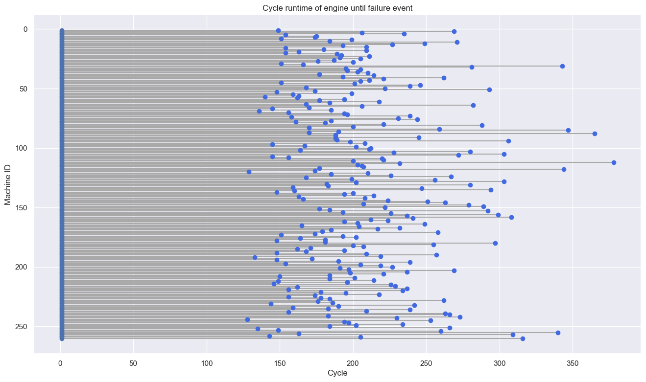
We assume that the observation time limit is 220 cycles so that when the machine is still active after 220 cycles then the machine will be considered right censored.
# Create status column
turbofan_df['status'] = turbofan_df['cycle'].apply(lambda x: False if x > 215 else True)
turbofan_df.head(5)
| cycle | operational_setting_1 | operational_setting_2 | operational_setting_3 | sensor_measurement_01 | sensor_measurement_02 | sensor_measurement_03 | sensor_measurement_04 | sensor_measurement_05 | sensor_measurement_06 | ... | sensor_measurement_13 | sensor_measurement_14 | sensor_measurement_15 | sensor_measurement_16 | sensor_measurement_17 | sensor_measurement_18 | sensor_measurement_19 | sensor_measurement_20 | sensor_measurement_21 | status | |
|---|---|---|---|---|---|---|---|---|---|---|---|---|---|---|---|---|---|---|---|---|---|
| machine_name | |||||||||||||||||||||
| 1 | 149 | 42.0017 | 0.8414 | 100.0 | 445.00 | 550.49 | 1366.01 | 1149.81 | 3.91 | 5.71 | ... | 2387.40 | 8066.19 | 9.4765 | 0.02 | 332 | 2212 | 100.0 | 10.45 | 6.2285 | True |
| 2 | 269 | 42.0047 | 0.8411 | 100.0 | 445.00 | 550.11 | 1368.75 | 1146.65 | 3.91 | 5.72 | ... | 2388.42 | 8110.26 | 9.4315 | 0.02 | 334 | 2212 | 100.0 | 10.56 | 6.2615 | False |
| 3 | 206 | 42.0073 | 0.8400 | 100.0 | 445.00 | 550.80 | 1356.97 | 1144.89 | 3.91 | 5.72 | ... | 2387.87 | 8082.25 | 9.4962 | 0.02 | 333 | 2212 | 100.0 | 10.46 | 6.3349 | True |
| 4 | 235 | 0.0030 | 0.0007 | 100.0 | 518.67 | 643.68 | 1605.86 | 1428.21 | 14.62 | 21.61 | ... | 2388.17 | 8215.14 | 8.5784 | 0.03 | 397 | 2388 | 100.0 | 38.47 | 22.9717 | False |
| 5 | 154 | 42.0049 | 0.8408 | 100.0 | 445.00 | 550.53 | 1364.82 | 1146.87 | 3.91 | 5.72 | ... | 2389.19 | 8151.36 | 9.4339 | 0.02 | 333 | 2212 | 100.0 | 10.74 | 6.3906 | True |
5 rows × 26 columns
Machine status
Trueindicates that the machine has failed within the observation time span whileFalseindicates the machine has not failed yet during the observation time span.
# Distribution of each status
turbofan_df['status'].value_counts()
True     173
False     87
Name: status, dtype: int64
Exploratory Data Analysis
The next step is to perform feature selection, which is the selection of variables as predictors that we want to include in the model.
turbofan_df.describe()
| cycle | operational_setting_1 | operational_setting_2 | sensor_measurement_01 | sensor_measurement_02 | sensor_measurement_03 | sensor_measurement_04 | sensor_measurement_05 | sensor_measurement_06 | sensor_measurement_07 | ... | sensor_measurement_11 | sensor_measurement_12 | sensor_measurement_13 | sensor_measurement_14 | sensor_measurement_15 | sensor_measurement_17 | sensor_measurement_18 | sensor_measurement_19 | sensor_measurement_20 | sensor_measurement_21 | |
|---|---|---|---|---|---|---|---|---|---|---|---|---|---|---|---|---|---|---|---|---|---|
| count | 260.000000 | 260.000000 | 260.000000 | 260.000000 | 260.000000 | 260.000000 | 260.000000 | 260.000000 | 260.000000 | 260.000000 | ... | 260.000000 | 260.000000 | 260.000000 | 260.000000 | 260.000000 | 260.000000 | 260.000000 | 260.000000 | 260.000000 | 260.000000 |
| mean | 206.765385 | 27.937113 | 0.598383 | 466.689346 | 575.619115 | 1425.801000 | 1218.674692 | 7.124231 | 10.386385 | 255.637115 | ... | 43.836038 | 240.824538 | 2364.920731 | 8105.652538 | 9.288340 | 349.815385 | 2242.073077 | 99.014654 | 18.644115 | 11.185072 |
| std | 46.782198 | 16.564435 | 0.324420 | 27.479073 | 36.085540 | 97.552983 | 114.934975 | 3.949434 | 5.864195 | 153.443600 | ... | 2.682455 | 144.687933 | 89.267941 | 74.714146 | 0.584163 | 25.629762 | 108.889934 | 3.732538 | 10.443101 | 6.261529 |
| min | 128.000000 | 0.000100 | 0.000000 | 445.000000 | 536.620000 | 1263.290000 | 1058.960000 | 3.910000 | 5.710000 | 136.990000 | ... | 37.210000 | 129.330000 | 2027.610000 | 7850.960000 | 8.486100 | 309.000000 | 1915.000000 | 84.930000 | 10.270000 | 6.164800 |
| 25% | 174.000000 | 10.003225 | 0.250650 | 445.000000 | 550.477500 | 1364.650000 | 1143.535000 | 3.910000 | 5.720000 | 138.277500 | ... | 42.650000 | 130.280000 | 2387.970000 | 8081.580000 | 8.753125 | 334.000000 | 2212.000000 | 100.000000 | 10.470000 | 6.283750 |
| 50% | 199.000000 | 41.998300 | 0.840000 | 445.000000 | 550.880000 | 1370.270000 | 1147.880000 | 3.910000 | 5.720000 | 139.165000 | ... | 42.770000 | 130.985000 | 2388.320000 | 8116.755000 | 9.414700 | 335.000000 | 2212.000000 | 100.000000 | 10.685000 | 6.390250 |
| 75% | 230.250000 | 42.002625 | 0.840100 | 489.050000 | 606.042500 | 1512.122500 | 1329.327500 | 10.520000 | 15.500000 | 392.595000 | ... | 46.070000 | 370.152500 | 2388.752500 | 8148.730000 | 9.456725 | 372.000000 | 2319.000000 | 100.000000 | 28.210000 | 16.925775 |
| max | 378.000000 | 42.007900 | 0.842000 | 518.670000 | 644.260000 | 1609.460000 | 1438.160000 | 14.620000 | 21.610000 | 551.980000 | ... | 48.510000 | 520.250000 | 2390.390000 | 8252.610000 | 11.045400 | 398.000000 | 2388.000000 | 100.000000 | 38.680000 | 23.153900 |
8 rows × 23 columns
turbofan_df.iloc[:,8:].head()
| sensor_measurement_05 | sensor_measurement_06 | sensor_measurement_07 | sensor_measurement_08 | sensor_measurement_09 | sensor_measurement_10 | sensor_measurement_11 | sensor_measurement_12 | sensor_measurement_13 | sensor_measurement_14 | sensor_measurement_15 | sensor_measurement_16 | sensor_measurement_17 | sensor_measurement_18 | sensor_measurement_19 | sensor_measurement_20 | sensor_measurement_21 | status | |
|---|---|---|---|---|---|---|---|---|---|---|---|---|---|---|---|---|---|---|
| machine_name | ||||||||||||||||||
| 1 | 3.91 | 5.71 | 137.76 | 2211.38 | 8307.72 | 1.02 | 42.77 | 129.55 | 2387.40 | 8066.19 | 9.4765 | 0.02 | 332 | 2212 | 100.0 | 10.45 | 6.2285 | True |
| 2 | 3.91 | 5.72 | 138.61 | 2212.32 | 8358.80 | 1.02 | 42.64 | 129.76 | 2388.42 | 8110.26 | 9.4315 | 0.02 | 334 | 2212 | 100.0 | 10.56 | 6.2615 | False |
| 3 | 3.91 | 5.72 | 138.08 | 2211.81 | 8329.26 | 1.02 | 42.85 | 130.02 | 2387.87 | 8082.25 | 9.4962 | 0.02 | 333 | 2212 | 100.0 | 10.46 | 6.3349 | True |
| 4 | 14.62 | 21.61 | 551.49 | 2388.17 | 9150.14 | 1.30 | 48.25 | 520.25 | 2388.17 | 8215.14 | 8.5784 | 0.03 | 397 | 2388 | 100.0 | 38.47 | 22.9717 | False |
| 5 | 3.91 | 5.72 | 138.48 | 2212.99 | 8397.52 | 1.02 | 42.67 | 130.05 | 2389.19 | 8151.36 | 9.4339 | 0.02 | 333 | 2212 | 100.0 | 10.74 | 6.3906 | True |
Check Uniqueness
Pertama kita akan memeriksa banyak nilai unik pada setiap kolom lalu kolom yang memiliki nilai unik yang sedikit akan diganti dengan tipe data kategori.
turbofan_df.nunique()
cycle                    133
operational_setting_1    165
operational_setting_2     62
operational_setting_3      2
sensor_measurement_01      6
sensor_measurement_02    188
sensor_measurement_03    257
sensor_measurement_04    251
sensor_measurement_05      6
sensor_measurement_06      8
sensor_measurement_07    209
sensor_measurement_08    177
sensor_measurement_09    259
sensor_measurement_10      8
sensor_measurement_11    123
sensor_measurement_12    198
sensor_measurement_13    152
sensor_measurement_14    258
sensor_measurement_15    247
sensor_measurement_16      2
sensor_measurement_17     27
sensor_measurement_18      6
sensor_measurement_19      2
sensor_measurement_20    135
sensor_measurement_21    253
status                     2
dtype: int64
Columns that can be changed to category type:
operational_setting_3,sensor_measurement_16
# Change to category
cat = ['operational_setting_3', 'sensor_measurement_16']

turbofan_df[cat] = turbofan_df[cat].astype('category')
turbofan_df.info()
<class 'pandas.core.frame.DataFrame'>
Int64Index: 260 entries, 1 to 260
Data columns (total 26 columns):
 #   Column                 Non-Null Count  Dtype
---  ------                 --------------  -----
 0   cycle                  260 non-null    int64
 1   operational_setting_1  260 non-null    float64
 2   operational_setting_2  260 non-null    float64
 3   operational_setting_3  260 non-null    category
 4   sensor_measurement_01  260 non-null    float64
 5   sensor_measurement_02  260 non-null    float64
 6   sensor_measurement_03  260 non-null    float64
 7   sensor_measurement_04  260 non-null    float64
 8   sensor_measurement_05  260 non-null    float64
 9   sensor_measurement_06  260 non-null    float64
 10  sensor_measurement_07  260 non-null    float64
 11  sensor_measurement_08  260 non-null    float64
 12  sensor_measurement_09  260 non-null    float64
 13  sensor_measurement_10  260 non-null    float64
 14  sensor_measurement_11  260 non-null    float64
 15  sensor_measurement_12  260 non-null    float64
 16  sensor_measurement_13  260 non-null    float64
 17  sensor_measurement_14  260 non-null    float64
 18  sensor_measurement_15  260 non-null    float64
 19  sensor_measurement_16  260 non-null    category
 20  sensor_measurement_17  260 non-null    int64
 21  sensor_measurement_18  260 non-null    int64
 22  sensor_measurement_19  260 non-null    float64
 23  sensor_measurement_20  260 non-null    float64
 24  sensor_measurement_21  260 non-null    float64
 25  status                 260 non-null    bool
dtypes: bool(1), category(2), float64(20), int64(3)
memory usage: 57.9 KB
Correlation Heatmap
We can check the correlation between columns of candidate predictors to see if there is a high correlation between predictors. Variables that have a high correlation with other variables need to be selected to avoid multicollinearity.
sns.heatmap(turbofan_df.corr()**2, annot = True,)
<AxesSubplot:>
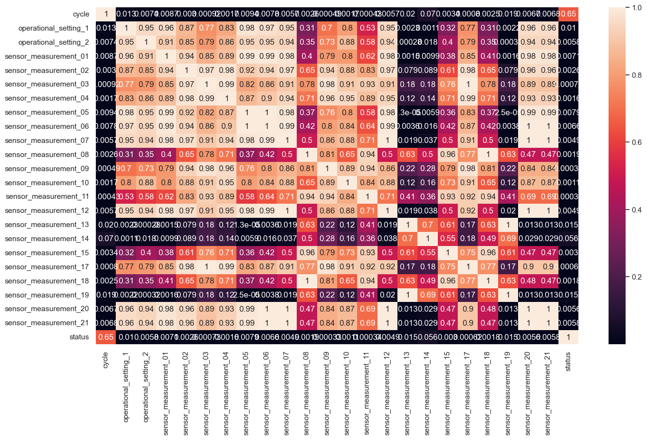
In the plot above, the correlation between variables looks quite high. In this case we will try to first select the columns
sensor_measurement_04,sensor_measurement_08,sensor_measurement_11,sensor_measurement_14.
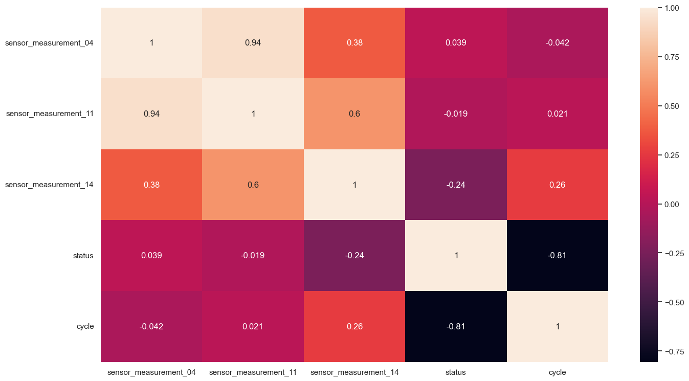
selected_columns = ['sensor_measurement_04','sensor_measurement_11','sensor_measurement_14']
cleaned_data = turbofan_df.loc[:, selected_columns + cat + ['status', 'cycle']]
sns.heatmap(cleaned_data.corr(), annot = True)
<AxesSubplot:>
Data Preparation for Modeling
The next step is to prepare the data for modeling. Things that need to be considered are:
- For columns with category type, One Hot Encoding needs to be done.
- For the target data, it needs to be written in the form of an array with each element is a tuple consisting of the machine status (True/False) and the time/cycle
# One Hot Encoding for Categorical Variable
from sksurv.preprocessing import OneHotEncoder

data_x = OneHotEncoder().fit_transform(cleaned_data.iloc[:, :-2])
data_x.head()
| sensor_measurement_04 | sensor_measurement_11 | sensor_measurement_14 | operational_setting_3=100.0 | sensor_measurement_16=0.03 | |
|---|---|---|---|---|---|
| machine_name | |||||
| 1 | 1149.81 | 42.77 | 8066.19 | 1.0 | 0.0 |
| 2 | 1146.65 | 42.64 | 8110.26 | 1.0 | 0.0 |
| 3 | 1144.89 | 42.85 | 8082.25 | 1.0 | 0.0 |
| 4 | 1428.21 | 48.25 | 8215.14 | 1.0 | 1.0 |
| 5 | 1146.87 | 42.67 | 8151.36 | 1.0 | 0.0 |
# Preprocessing for target variable

data_y = list(cleaned_data.loc[:, ["status", "cycle"]].itertuples(index = None, name = None))
data_y = np.array(data_y, dtype=[('status', bool), ('cycle', float)])
data_y[:5]
array([( True, 149.), (False, 269.), ( True, 206.), (False, 235.),
       ( True, 154.)], dtype=[('status', '?'), ('cycle', '<f8')])
# Preprocessing for target variable

target_data = list(cleaned_data.loc[:, ["status", "cycle"]].itertuples(index = None, name = None))
target_data = np.array(target_data, dtype=[('status', bool), ('cycle', float)])
target_data[:5]
array([( True, 149.), (False, 269.), ( True, 206.), (False, 235.),
       ( True, 154.)], dtype=[('status', '?'), ('cycle', '<f8')])
Kaplan-Meier Estimator
From the data we have above, we can build a survival function Kaplan Meier Estimator. The Kaplan Meier Estimator is built by calculating the probability of observations that survive (do not experience events) at each time. Mathematically, the Kaplan Meier Estimator can be written as follows: \(S(t) = \prod_{j=1}^{t} \frac{n_j - d_j}{n_j}\) where $n_j$ is the number of subjects at time $j$ and $d_j$ is the number of subjects that experienced the event.
from lifelines import KaplanMeierFitter

# Instantiate Kaplan Meier object
kmf = KaplanMeierFitter()

# Fit Kaplan Meier estimator
kmf.fit(durations=target_data['cycle'], event_observed=target_data['status'])
<lifelines.KaplanMeierFitter:"KM_estimate", fitted with 260 total observations, 87 right-censored observations>
# Plot survival function with confidence intervals
kmf.plot_survival_function()

plt.title("Kaplan-Meier Estimator")
plt.ylabel("est. probability of survival $\hat{S}(t)$")
plt.xlabel("time $t$")

plt.show()
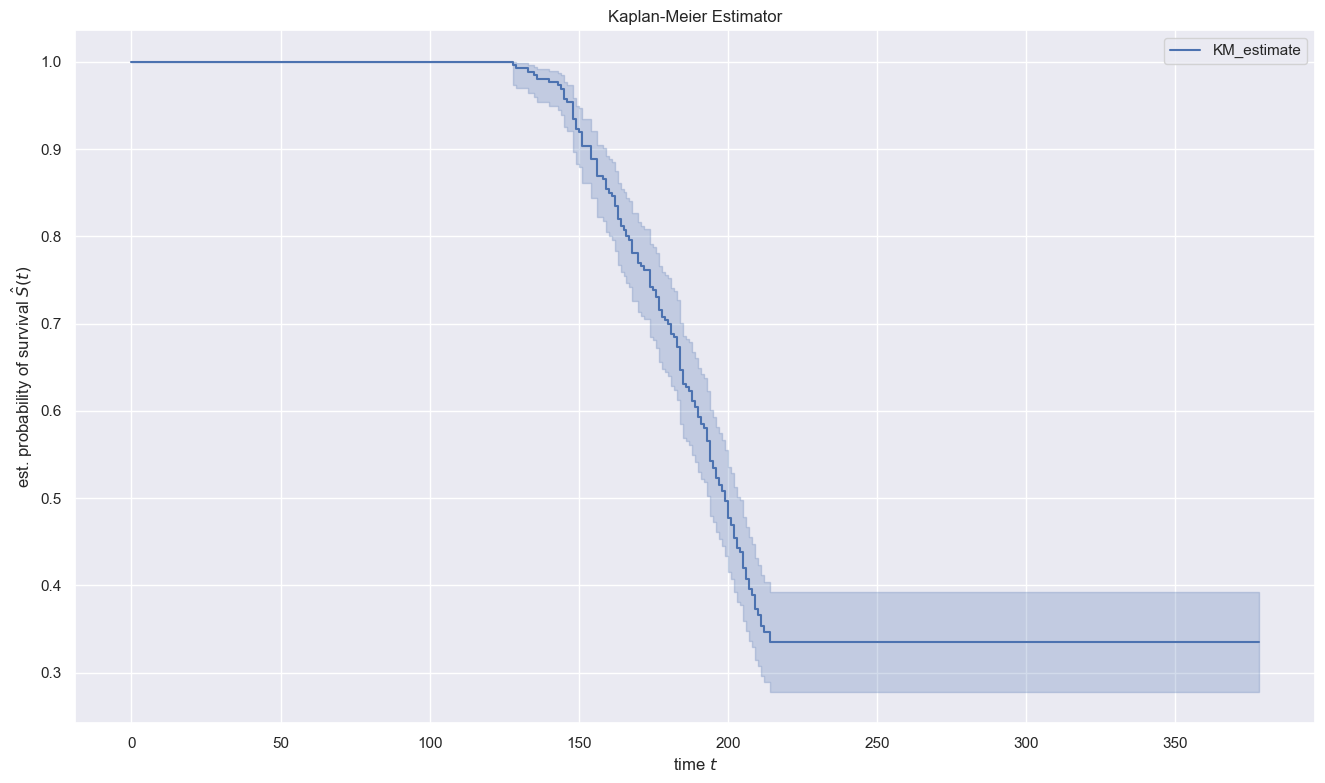
Interpretation:
- Until the time $t=125$ the value of $S(t)=1$ which indicates that all machines are still running until the 125th cycle
- When $t=175$ the value of $S(t)$ is around 0.75 indicating that after about 75% the engine is still running until the 175th cycle
- The chance of a engine still having not failed is 50% at cycle 190.
Compare Survival Time for Each value in categorical columns
We have learned how to construct a survival function using the Kaplan Meier Estimator. Sometimes we want to do a comparison on whether different categories/treatments will affect the survival of our subjects.
For example, in cleaned_data we have two columns that have category types operational_setting_3 and sensor_measurement_16. Let’s check the number of unique values in these two columns
In this section, we will compare the distribution of survival time for each category in every categorical columns. From the distribution we hope that we can determine if there is a difference distribution for each category or not.
os3_unique = list(cleaned_data['operational_setting_3'].unique())
sm16_unique = list(cleaned_data['sensor_measurement_16'].unique())
print(f'Unique values operational_setting_3: {os3_unique}')
print(f'Unique values sensor_measurement_16: {sm16_unique}')
Unique values operational_setting_3: [100.0, 60.0]
Unique values sensor_measurement_16: [0.02, 0.03]
Now we will compare the distribution of the survival function between the values 100 and 60 in the operational_setting_3.
# plt.xlabel callable bugfix
import matplotlib.pyplot as plt
from importlib import reload
plt=reload(plt)

fig, ax = plt.subplots(1, 1, sharex='col', sharey='row')

# Mask for operational_setting_3
fullos3 = (cleaned_data['operational_setting_3'] == 100)

kmf = KaplanMeierFitter()
kmf.fit(durations=cleaned_data[fullos3]['cycle'], event_observed=cleaned_data[fullos3]['status'])
kmf.plot_survival_function(ax=ax)

kmf = KaplanMeierFitter()
kmf.fit(durations=cleaned_data[~fullos3]['cycle'], event_observed=cleaned_data[~fullos3]['status'])
kmf.plot_survival_function(ax=ax)


plt.title(f"Kaplan-Meier Estimator for both operational settings 3")
plt.legend(loc="best")
plt.xlabel('cycles')
plt.ylabel("est. probability of survival $\hat{S}(t)$")
plt.show()
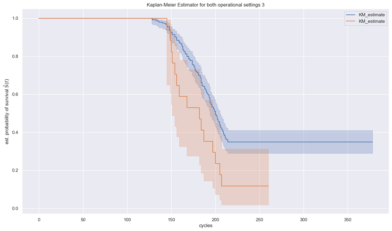
Please notice that leaving confidence intervals (shaded areas) left aside, there is a broad gap between the survival curves. With the confidence intervals in the picture however, the overlapping confidence interval areas show that the observed gap might not indicate real differences in the survival functions. There is no significant difference that could be determined.
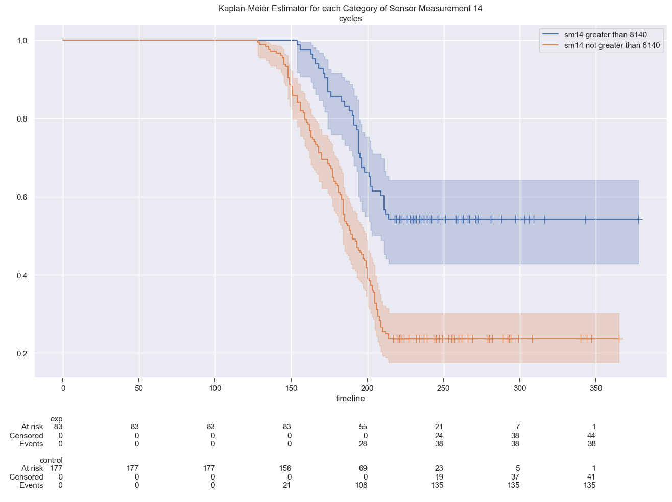
A different picture is that of two groups separated by a threshold of sensor measurements no 14 where there are significant different survival function curves:
# plt.xlabel callable bugfix
import matplotlib.pyplot as plt
from importlib import reload
plt=reload(plt)

threshold = 8140

fig, ax = plt.subplots(1, 1, sharex='col', sharey='row')

# Mask
sm14 = (cleaned_data['sensor_measurement_14'] > threshold)

kmf_exp = KaplanMeierFitter()
kmf_exp.fit(durations=cleaned_data[sm14]['cycle'], event_observed=cleaned_data[sm14]['status'], label='exp')
kmf_exp.plot_survival_function(ax=ax, show_censors=True, ci_legend=True,
                               label='sm14 greater than ' + str(threshold)
                              )

kmf_control = KaplanMeierFitter()
kmf_control.fit(durations=cleaned_data[~sm14]['cycle'], event_observed=cleaned_data[~sm14]['status'], label='control')
kmf_control.plot_survival_function(ax=ax, show_censors=True, ci_legend=True,
                                   label='sm14 not greater than ' + str(threshold)
                                  )


from lifelines.plotting import add_at_risk_counts
add_at_risk_counts(kmf_exp, kmf_control, ax=ax)

plt.title(f"Kaplan-Meier Estimator for each Category of Sensor Measurement 14")
plt.ylabel("est. probability of survival $\hat{S}(t)$")
plt.xlabel('cycles')
plt.show()
Log-Rank Test
In the previous section, we compared the distribution of survival functions by visualization. However, sometimes further statistical tests are required to determine whether the two distributions can be said to be the same or significantly different. To perform these tests, we can use the Log-. Rank Test with the usual statistical hypotheses.
$H_{0}$ : The distribution of the two survival functions is the same
$H_{1}$ : The distribution of the two survival functions is different
from sksurv.compare import compare_survival

cat.append('sensor_measurement_14')

p_value_list = []
for column in cat:
    p_value = compare_survival(data_y, turbofan_df[column])[1]
    p_value_list.append(p_value)

result = pd.DataFrame({'columns': cat, 'p-value': p_value_list}).set_index('columns')
result['conclusion'] = result['p-value'].apply(lambda x: "significant" if x < 0.05 else "not significant")
result
| p-value | conclusion | |
|---|---|---|
| columns | ||
| operational_setting_3 | 5.391624e-03 | significant |
| sensor_measurement_16 | 7.368610e-02 | not significant |
| sensor_measurement_14 | 4.966909e-145 | significant |
cleaned_data
| sensor_measurement_04 | sensor_measurement_11 | sensor_measurement_14 | operational_setting_3 | sensor_measurement_16 | status | cycle | |
|---|---|---|---|---|---|---|---|
| machine_name | |||||||
| 1 | 1149.81 | 42.77 | 8066.19 | 100.0 | 0.02 | True | 149 |
| 2 | 1146.65 | 42.64 | 8110.26 | 100.0 | 0.02 | False | 269 |
| 3 | 1144.89 | 42.85 | 8082.25 | 100.0 | 0.02 | True | 206 |
| 4 | 1428.21 | 48.25 | 8215.14 | 100.0 | 0.03 | False | 235 |
| 5 | 1146.87 | 42.67 | 8151.36 | 100.0 | 0.02 | True | 154 |
| ... | ... | ... | ... | ... | ... | ... | ... |
| 256 | 1425.84 | 48.36 | 8128.22 | 100.0 | 0.03 | True | 163 |
| 257 | 1146.53 | 42.70 | 8171.37 | 100.0 | 0.02 | False | 309 |
| 258 | 1326.79 | 46.08 | 8124.16 | 100.0 | 0.03 | True | 143 |
| 259 | 1149.97 | 42.73 | 8075.91 | 100.0 | 0.02 | True | 205 |
| 260 | 1145.52 | 42.50 | 8185.35 | 100.0 | 0.02 | False | 316 |
260 rows × 7 columns
cleaned_data[sm14]['cycle'].count()
83
cleaned_data[~sm14]['cycle'].count()
177
# Import logrank_test
from lifelines.statistics import logrank_test

sm16 = (cleaned_data['sensor_measurement_16'] == 0.02)

# Run log-rank test to compare groups by survival function
mask_dict = {'sensor_measurement_14': sm14, 'sensor_measurement_16': sm16, 'operational_setting_3': fullos3}
p_value_list = []

for item in mask_dict.items():
    lrt = logrank_test(durations_A = cleaned_data[item[1]]['cycle'],
                       durations_B = cleaned_data[~item[1]]['cycle'],
                       event_observed_A = cleaned_data[item[1]]['status'],
                       event_observed_B = cleaned_data[~item[1]]['status'])
    p_value_list.append(lrt.p_value)

test_results = pd.DataFrame({'feature': mask_dict.keys(), 'p-value': p_value_list}).set_index('feature')
test_results['conclusion'] = test_results['p-value'].apply(lambda x: "significant" if x < 0.05 else "not significant")
test_results
| p-value | conclusion | |
|---|---|---|
| feature | ||
| sensor_measurement_14 | 5.276097e-07 | significant |
| sensor_measurement_16 | 7.368610e-02 | not significant |
| operational_setting_3 | 5.391624e-03 | significant |
Conclusion : For the features operational_setting_3 and sensor_measurement_14 there are significant differences in the survival function between the groups.
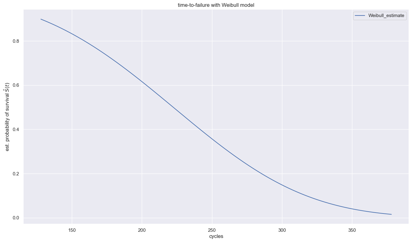
Weibull Distribution
Lets fit the Weibull distribution as a parametric model for our time-to-event data. We use survival regression to make inferences about how covariates affect the survival function and select the best survival model for our data.
# plt.xlabel callable bugfix
import matplotlib.pyplot as plt
from importlib import reload
plt=reload(plt)

# Import WeibullFitter class
from lifelines import WeibullFitter

# Instantiate WeibullFitter
wb = WeibullFitter()

# Fit data to wb
wb.fit(data_y["cycle"], data_y["status"])

# Plot survival function
wb.survival_function_.plot()
plt.title(f"time-to-failure with Weibull model")
plt.ylabel("est. probability of survival $\hat{S}(t)$")
plt.xlabel('cycles')

plt.show()
threshold = 8100

# Mask for operational_setting_3
sm14 = (cleaned_data['sensor_measurement_14'] > threshold)

# Fit to sm14 greater than 8140
wb.fit(#durations=prison[parole]['week'], event_observed=prison[parole]['arrest']
      durations=cleaned_data[sm14]['cycle'], event_observed=cleaned_data[sm14]['status']
       #, label='exp'
      )

# Print rho
print("The rho_ parameter of group sm14 greater than 8140: ", wb.rho_)

# Fit to engines sm14 lower equal than 8140
wb.fit(durations=cleaned_data[~sm14]['cycle'], event_observed=cleaned_data[~sm14]['status'])

# Print rho
print("The rho_ parameter of group sm14 lower equal than 8140 survival function is: ", wb.rho_)
The rho_ parameter of group sm14 greater than 8140:  3.278560362707543
The rho_ parameter of group sm14 lower equal than 8140 survival function is:  3.8024815134050174
Both rho values are much larger than 1, which indicates that both groups’ rate of event increases as time goes on.
Multiple covariates with the Weibull Accelerated Failure Time model (Weibull AFT)
# Import WeibullAFTFitter and instantiate
from lifelines import WeibullAFTFitter
aft = WeibullAFTFitter()

# Fit heart_patients data into aft
aft.fit(cleaned_data, duration_col='cycle', event_col='status')

# Print the summary
print(aft.summary)
                                    coef     exp(coef)   se(coef)  \
param   covariate
lambda_ operational_setting_3  -0.057131  9.444701e-01   0.014956
        sensor_measurement_04  -0.009645  9.904010e-01   0.002959
        sensor_measurement_11   0.475113  1.608197e+00   0.147451
        sensor_measurement_14   0.003070  1.003074e+00   0.000585
        sensor_measurement_16  -0.564594  5.685911e-01  13.080660
        Intercept             -22.867489  1.171590e-10   4.716158
rho_    Intercept               1.306051  3.691566e+00   0.058606

                               coef lower 95%  coef upper 95%  \
param   covariate
lambda_ operational_setting_3       -0.086444       -0.027818
        sensor_measurement_04       -0.015446       -0.003845
        sensor_measurement_11        0.186115        0.764112
        sensor_measurement_14        0.001924        0.004215
        sensor_measurement_16      -26.202217       25.073029
        Intercept                  -32.110988      -13.623990
rho_    Intercept                    1.191185        1.420916

                               exp(coef) lower 95%  exp(coef) upper 95%  \
param   covariate
lambda_ operational_setting_3         9.171866e-01         9.725653e-01
        sensor_measurement_04         9.846729e-01         9.961623e-01
        sensor_measurement_11         1.204560e+00         2.147087e+00
        sensor_measurement_14         1.001926e+00         1.004224e+00
        sensor_measurement_16         4.173705e-12         7.746014e+10
        Intercept                     1.133379e-14         1.211090e-06
rho_    Intercept                     3.290980e+00         4.140913e+00

                               cmp to          z              p    -log2(p)
param   covariate
lambda_ operational_setting_3     0.0  -3.819968   1.334689e-04   12.871209
        sensor_measurement_04     0.0  -3.259247   1.117084e-03    9.806046
        sensor_measurement_11     0.0   3.222178   1.272201e-03    9.618458
        sensor_measurement_14     0.0   5.250649   1.515641e-07   22.653569
        sensor_measurement_16     0.0  -0.043162   9.655720e-01    0.050544
        Intercept                 0.0  -4.848754   1.242393e-06   19.618447
rho_    Intercept                 0.0  22.285300  5.131147e-110  363.052809
# Calculate the exponential of sensor measurement 11 coefficient
exp_sm11 = np.exp(aft.params_.loc['lambda_'].loc['sensor_measurement_11'])
print('When sensor_measurement_11 increases by 1, the average survival duration changes by a factor of', exp_sm11)
When sensor_measurement_11 increases by 1, the average survival duration changes by a factor of 1.608196633553678
# Fit data to aft
aft.fit(cleaned_data, duration_col='cycle', event_col='status')

# Plot partial effects of prio
#aft.plot_partial_effects_on_outcome(  covariates='sensor_measurement_14',   values=np.arange(8090, 8170, 15))
aft.plot_partial_effects_on_outcome(  covariates='sensor_measurement_11',   values=np.arange(42, 45, 0.5))

plt.axvline(x=250,ls="--",c=".5")

plt.title(f"Weibull baseline model vs. varied values of sensor measurements 11")
plt.ylabel("survival probability")
plt.xlabel('cycles')
plt.show()
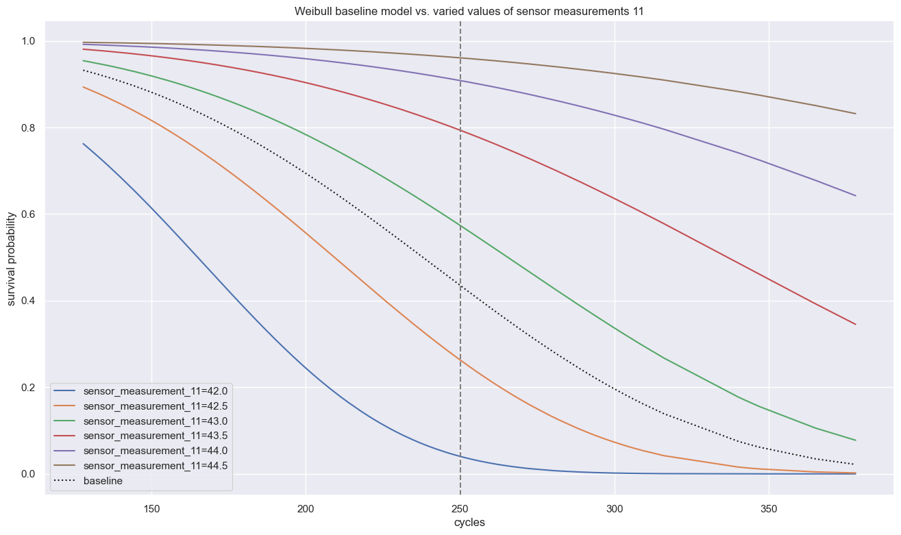
Visualized in this ‘partial effects plot’ above, we can see how sensor measurements 11 determine survival times significantly while every other covariate holding equal, even half a point difference of 42.5 vs. 43.0 at cycle 250 halves the survival probability.
# Predict median of new data
aft_pred = aft.predict_median(cleaned_data)

# Print average predicted time to arrest
print("On average, the median number of cycles for an engine to fail is: ", np.mean(aft_pred))
On average, the median number of cycles for an engine to fail is: 226.12247644680892
In case we want use predictions of our models we have to validate/invalidate our models, which can happen numerically and graphically. The regular way to compare and validate different models is the Akaike information criterion (AIC) with which the best fitting model can be easily determined.
from lifelines.fitters.exponential_fitter import ExponentialFitter
from lifelines.fitters.log_normal_fitter import LogNormalFitter
from lifelines.fitters.log_logistic_fitter import LogLogisticFitter

# Instantiate each fitter
wb = WeibullFitter()
exp = ExponentialFitter()
lognorm = LogNormalFitter()
loglog = LogLogisticFitter()

# Fit to data
for model in [wb, exp, lognorm, loglog]:
      model.fit(durations=cleaned_data[sm14]['cycle'], event_observed=cleaned_data[sm14]['status'] )
      # Print AIC
      print(model.__class__.__name__, model.AIC_)
WeibullFitter 1311.250877441705
ExponentialFitter 1440.767027487693
LogNormalFitter 1269.5021223158335
LogLogisticFitter 1274.537494437834
How good is the fit visually?
fig, axes = plt.subplots(2, 2, figsize=(10, 8))
axes = axes.reshape(4,)

for i, model in enumerate([WeibullFitter(), LogNormalFitter(), LogLogisticFitter(), ExponentialFitter()]):
    model.fit(durations=cleaned_data[sm14]['cycle'], event_observed=cleaned_data[sm14]['status'] )
    qq_plot(model, ax=axes[i])

plt.suptitle(f"QQ Plot of Fitted models of different distributions of those engines with Sensor Measurement 14 above threshold {threshold}" )
plt.show()
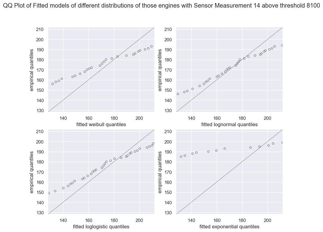
The LogNormal Fitted Model fits the data best and reasonable well; minor tail separation from the diagonal line is expected and within acceptable bounds.
data_x = data_x[data_x.columns[~data_x.columns.isin(["sensor_measurement_16=0.03"])]]
Cox Propotional Hazard
The hazard function $ h(t) $ describes the probability that the event of interest will occur at a given time if individuals survive to that time. The hazard rates along this function are the instantaneous rates for the occurrence of the event. \(h(t) = h_{0}(t) e^{\beta_{1}x_{1} + \beta_{2}x_{2} + ... + \beta_{n}x_{n}}\)
The Cox Propotional Hazard (CoxPH) model is a semiparametric model that will predict the value of the hazard rate which consists of the following components:
-
Non-parametric $h_{0}(t)$ (baseline hazard) : Characterization of how the hazard function changes over time. This baseline hazard can also be interpreted as an intercept in the regression problem
Parametric $e^{\beta_{1}x_{1} + \beta_{2}x_{2} + … + \beta_{n}x_{n}}$ : Characterization of how the hazard function changes based on covariate conditions (variables involved in the model)
The survival function based on the above model can be obtained through the hazard function, which are closely related: \(S(t) = e^{-\int{h(t)}} dt\)
regularization alpha = 1e-4
from sksurv.linear_model import CoxPHSurvivalAnalysis

# Define model
estimator = CoxPHSurvivalAnalysis(verbose = 10)

# Fitting model
estimator.fit(data_x, data_y)
iter      1: update = [-0.02672891  1.30951039  0.00897907 -6.14944208]
iter      1: loss = 3.4407602869
iter      2: update = [ 0.00043914 -0.0348166   0.00100936 -0.27206197]
iter      2: loss = 3.4389450619
iter      3: update = [-1.01083581e-05  6.09861343e-04 -3.68327372e-06 -1.80823588e-02]
iter      3: loss = 3.4389378698
iter      4: update = [ 1.34113910e-08 -7.92317762e-07  2.80717143e-09 -1.08672544e-04]
iter      4: loss = 3.4389378694
iter      4: optimization converged


CoxPHSurvivalAnalysis(verbose=10)
cleaned_data = cleaned_data.drop('sensor_measurement_16', axis=1)
# Import CoxPHFitter class
from lifelines import CoxPHFitter

# Instantiate CoxPHFitter class cph
cph = CoxPHFitter(
    #penalizer=0.001
)

# Fit cph to data
cph.fit(df=cleaned_data, duration_col="cycle", event_col="status")

# Print model summary
print(cph.summary)
                           coef  exp(coef)  se(coef)  coef lower 95%  \
covariate
sensor_measurement_04  0.026635   1.026993  0.009872        0.007286
sensor_measurement_11 -1.291693   0.274805  0.515289       -2.301640
sensor_measurement_14 -0.010052   0.989998  0.002043       -0.014057
operational_setting_3  0.162776   1.176773  0.053030        0.058840

                       coef upper 95%  exp(coef) lower 95%  \
covariate
sensor_measurement_04        0.045984             1.007312
sensor_measurement_11       -0.281746             0.100095
sensor_measurement_14       -0.006047             0.986041
operational_setting_3        0.266712             1.060605

                       exp(coef) upper 95%  cmp to         z             p  \
covariate
sensor_measurement_04             1.047058     0.0  2.697954  6.976709e-03
sensor_measurement_11             0.754465     0.0 -2.506737  1.218513e-02
sensor_measurement_14             0.993971     0.0 -4.919302  8.685343e-07
operational_setting_3             1.305664     0.0  3.069527  2.143978e-03

                        -log2(p)
covariate
sensor_measurement_04   7.163238
sensor_measurement_11   6.358734
sensor_measurement_14  20.134914
operational_setting_3   8.865494
The hazard ratio is exp(coef) which is e to the power of a coefficient. It indicates how much the baseline hazard changes with a one-unit change in the covariate.
So with one unit increase in operational_setting_3 the hazard changes by a factor of 1.137, a 13.7% increase compared to the baseline hazard.
All four covariates are statistically significant as per column p, indicating that there is a strong correlation between the changes in all covariates and the hazards.
# Coef model
pd.Series(estimator.coef_, index = data_x.columns)
sensor_measurement_04          0.026300
sensor_measurement_11         -1.275303
sensor_measurement_14         -0.009985
operational_setting_3=100.0    6.439695
dtype: float64
Interpretation:
- Every one unit increase in
sensor_measurement_04will increase the hazard rate by $e^{0.02} = 1.02$ assuming no changes in other covariates - Every one unit increase in
sensor_measurement_11will reduce the hazard rate by $e^{-1.13} = 0. 32$ assuming no change in the other covariates - Using
operational_setting_3= 100 will increase the hazard rate by $e^{6.26} = 523.21$ compared tooperational_setting_3= 60
# Assign summary to summary_df
summary_df = cph.summary

# Create new column of survival time ratios
summary_df["surv_ratio"] = 1 / summary_df['exp(coef)']

summary_df
| coef | exp(coef) | se(coef) | coef lower 95% | coef upper 95% | exp(coef) lower 95% | exp(coef) upper 95% | cmp to | z | p | -log2(p) | surv_ratio | |
|---|---|---|---|---|---|---|---|---|---|---|---|---|
| covariate | ||||||||||||
| sensor_measurement_04 | 0.026635 | 1.026993 | 0.009872 | 0.007286 | 0.045984 | 1.007312 | 1.047058 | 0.0 | 2.697954 | 6.976709e-03 | 7.163238 | 0.973717 |
| sensor_measurement_11 | -1.291693 | 0.274805 | 0.515289 | -2.301640 | -0.281746 | 0.100095 | 0.754465 | 0.0 | -2.506737 | 1.218513e-02 | 6.358734 | 3.638942 |
| sensor_measurement_14 | -0.010052 | 0.989998 | 0.002043 | -0.014057 | -0.006047 | 0.986041 | 0.993971 | 0.0 | -4.919302 | 8.685343e-07 | 20.134914 | 1.010103 |
| operational_setting_3 | 0.162776 | 1.176773 | 0.053030 | 0.058840 | 0.266712 | 1.060605 | 1.305664 | 0.0 | 3.069527 | 2.143978e-03 | 8.865494 | 0.849782 |
# Print surv_ratio for prio
survivalratio = summary_df.loc['sensor_measurement_04', "surv_ratio"]
survivalratio
0.973716525421316
TimeToFailureChange = survivalratio - 1
TimeToFailureChange
-0.026283474578683963
print(f'Time-to-failure changes by {TimeToFailureChange * 100:.2f} %')
Time-to-failure changes by -2.63 %
So the impact on survival time with a one-unit increase in sensor_measurement_04 is more than negative 2 percent.
covars = list(summary_df["surv_ratio"].index)
covars
['sensor_measurement_04',
 'sensor_measurement_11',
 'sensor_measurement_14',
 'operational_setting_3']
sorted(covars)
['operational_setting_3',
 'sensor_measurement_04',
 'sensor_measurement_11',
 'sensor_measurement_14']
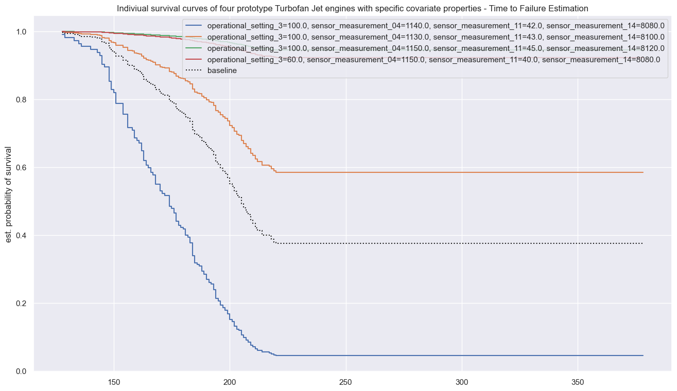
# Plot partial effects
cph.plot_partial_effects_on_outcome(covariates=sorted(covars),
         values=[[100.0,1140,42,8080],
                 [100.0,1130,43,8100],
                 [100.0,1150,45,8120],
                 [60,   1150,40,8080]])

# Show plot
plt.title("Indiviual survival curves of four prototype Turbofan Jet engines with specific covariate properties - Time to Failure Estimation" )
plt.ylabel("est. probability of survival")
#plt.xlabel("cycles")
plt.legend(loc="upper right")
plt.show()
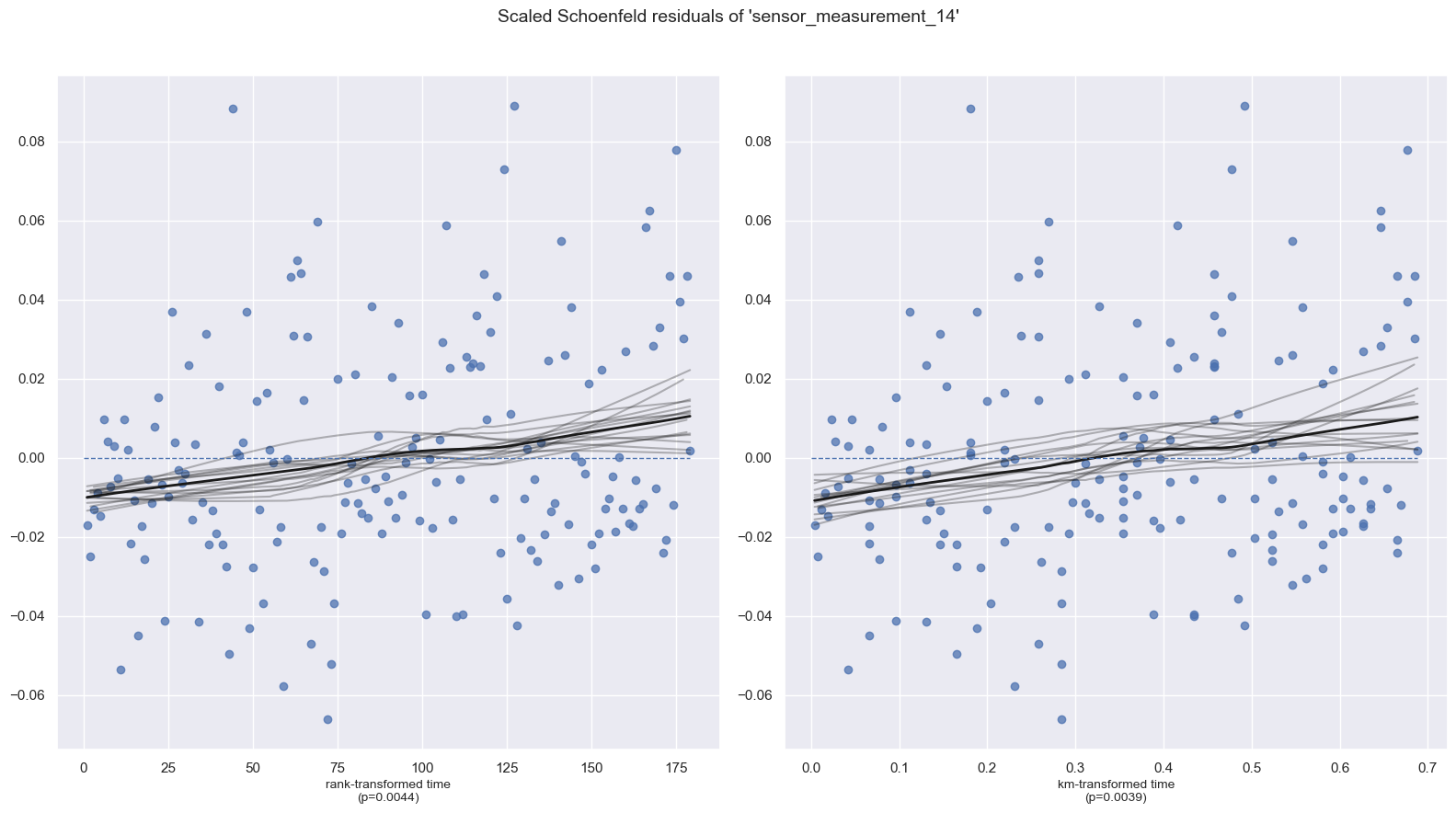
# Check PH assumption
print(cph.check_assumptions(training_df=cleaned_data, p_value_threshold=0.05, show_plots=True))
The ``p_value_threshold`` is set at 0.05. Even under the null hypothesis of no violations, some
covariates will be below the threshold by chance. This is compounded when there are many covariates.
Similarly, when there are lots of observations, even minor deviances from the proportional hazard
assumption will be flagged.

With that in mind, it's best to use a combination of statistical tests and visual tests to determine
the most serious violations. Produce visual plots using ``check_assumptions(..., show_plots=True)``
and looking for non-constant lines. See link [A] below for a full example.
| null_distribution | chi squared |
|---|---|
| degrees_of_freedom | 1 |
| model | <lifelines.CoxPHFitter: fitted with 260 total ... |
| test_name | proportional_hazard_test |
| test_statistic | p | -log2(p) | ||
|---|---|---|---|---|
| operational_setting_3 | km | 0.87 | 0.35 | 1.51 |
| rank | 0.95 | 0.33 | 1.60 | |
| sensor_measurement_04 | km | 1.58 | 0.21 | 2.26 |
| rank | 1.66 | 0.20 | 2.34 | |
| sensor_measurement_11 | km | 2.10 | 0.15 | 2.77 |
| rank | 2.20 | 0.14 | 2.86 | |
| sensor_measurement_14 | km | 8.35 | <0.005 | 8.02 |
| rank | 8.12 | <0.005 | 7.84 |
1. Variable 'sensor_measurement_14' failed the non-proportional test: p-value is 0.0039.

   Advice 1: the functional form of the variable 'sensor_measurement_14' might be incorrect. That
is, there may be non-linear terms missing. The proportional hazard test used is very sensitive to
incorrect functional forms. See documentation in link [D] below on how to specify a functional form.

   Advice 2: try binning the variable 'sensor_measurement_14' using pd.cut, and then specify it in
`strata=['sensor_measurement_14', ...]` in the call in `.fit`. See documentation in link [B] below.

   Advice 3: try adding an interaction term with your time variable. See documentation in link [C]
below.


   Bootstrapping lowess lines. May take a moment...


---
[A]  https://lifelines.readthedocs.io/en/latest/jupyter_notebooks/Proportional%20hazard%20assumption.html
[B]  https://lifelines.readthedocs.io/en/latest/jupyter_notebooks/Proportional%20hazard%20assumption.html#Bin-variable-and-stratify-on-it
[C]  https://lifelines.readthedocs.io/en/latest/jupyter_notebooks/Proportional%20hazard%20assumption.html#Introduce-time-varying-covariates
[D]  https://lifelines.readthedocs.io/en/latest/jupyter_notebooks/Proportional%20hazard%20assumption.html#Modify-the-functional-form
[E]  https://lifelines.readthedocs.io/en/latest/jupyter_notebooks/Proportional%20hazard%20assumption.html#Stratification

[[<AxesSubplot:xlabel='rank-transformed time\n(p=0.0044)'>, <AxesSubplot:xlabel='km-transformed time\n(p=0.0039)'>]]
Stratify sm14 and redo straified COXPH fitting
cleaned_strata_data = cleaned_data.copy()
cleaned_data.sensor_measurement_14.describe()
count     260.000000
mean     8105.652538
std        74.714146
min      7850.960000
25%      8081.580000
50%      8116.755000
75%      8148.730000
max      8252.610000
Name: sensor_measurement_14, dtype: float64
cleaned_strata_data
| sensor_measurement_04 | sensor_measurement_11 | sensor_measurement_14 | operational_setting_3 | status | cycle | |
|---|---|---|---|---|---|---|
| machine_name | ||||||
| 1 | 1149.81 | 42.77 | 8066.19 | 100.0 | True | 149 |
| 2 | 1146.65 | 42.64 | 8110.26 | 100.0 | False | 269 |
| 3 | 1144.89 | 42.85 | 8082.25 | 100.0 | True | 206 |
| 4 | 1428.21 | 48.25 | 8215.14 | 100.0 | False | 235 |
| 5 | 1146.87 | 42.67 | 8151.36 | 100.0 | True | 154 |
| ... | ... | ... | ... | ... | ... | ... |
| 256 | 1425.84 | 48.36 | 8128.22 | 100.0 | True | 163 |
| 257 | 1146.53 | 42.70 | 8171.37 | 100.0 | False | 309 |
| 258 | 1326.79 | 46.08 | 8124.16 | 100.0 | True | 143 |
| 259 | 1149.97 | 42.73 | 8075.91 | 100.0 | True | 205 |
| 260 | 1145.52 | 42.50 | 8185.35 | 100.0 | False | 316 |
260 rows × 6 columns
cph2 = CoxPHFitter()
cph2.fit(df=cleaned_strata_data, duration_col="cycle", event_col="status",
         #strata=['sm14_strata'],
         formula="bs(sensor_measurement_14, df=3, lower_bound=7850, upper_bound=8300) + sensor_measurement_04 + sensor_measurement_11 + operational_setting_3"
        )
<lifelines.CoxPHFitter: fitted with 260 total observations, 81 right-censored observations>
cph2.print_summary(3)
sns.set(rc = {'figure.figsize':(7,7)})
cph2.plot()
plt.show()
| model | lifelines.CoxPHFitter |
|---|---|
| duration col | 'cycle' |
| event col | 'status' |
| baseline estimation | breslow |
| number of observations | 260 |
| number of events observed | 179 |
| partial log-likelihood | -891.762 |
| time fit was run | 2022-09-17 08:02:35 UTC |
| coef | exp(coef) | se(coef) | coef lower 95% | coef upper 95% | exp(coef) lower 95% | exp(coef) upper 95% | cmp to | z | p | -log2(p) | |
|---|---|---|---|---|---|---|---|---|---|---|---|
| bs(sensor_measurement_14, df=3, lower_bound=7850, upper_bound=8300)[1] | 0.931 | 2.537 | 2.994 | -4.937 | 6.799 | 0.007 | 896.764 | 0.000 | 0.311 | 0.756 | 0.404 |
| bs(sensor_measurement_14, df=3, lower_bound=7850, upper_bound=8300)[2] | -4.767 | 0.009 | 2.662 | -9.984 | 0.451 | 0.000 | 1.570 | 0.000 | -1.791 | 0.073 | 3.769 |
| bs(sensor_measurement_14, df=3, lower_bound=7850, upper_bound=8300)[3] | -2.244 | 0.106 | 2.345 | -6.840 | 2.351 | 0.001 | 10.500 | 0.000 | -0.957 | 0.338 | 1.563 |
| operational_setting_3[T.100.0] | 6.298 | 543.528 | 2.649 | 1.107 | 11.489 | 3.025 | 97671.295 | 0.000 | 2.378 | 0.017 | 5.844 |
| sensor_measurement_04 | 0.027 | 1.027 | 0.010 | 0.008 | 0.046 | 1.008 | 1.047 | 0.000 | 2.725 | 0.006 | 7.281 |
| sensor_measurement_11 | -1.298 | 0.273 | 0.514 | -2.306 | -0.290 | 0.100 | 0.749 | 0.000 | -2.523 | 0.012 | 6.425 |
<div>
| Concordance | 0.650 |
|---|---|
| Partial AIC | 1795.525 |
| log-likelihood ratio test | 39.294 on 6 df |
| -log2(p) of ll-ratio test | 20.605 |
</div>

import warnings
warnings.simplefilter(action='ignore', category=FutureWarning)

cph2.check_assumptions(cleaned_strata_data)
The ``p_value_threshold`` is set at 0.01. Even under the null hypothesis of no violations, some
covariates will be below the threshold by chance. This is compounded when there are many covariates.
Similarly, when there are lots of observations, even minor deviances from the proportional hazard
assumption will be flagged.

With that in mind, it's best to use a combination of statistical tests and visual tests to determine
the most serious violations. Produce visual plots using ``check_assumptions(..., show_plots=True)``
and looking for non-constant lines. See link [A] below for a full example.
| null_distribution | chi squared |
|---|---|
| degrees_of_freedom | 1 |
| model | <lifelines.CoxPHFitter: fitted with 260 total ... |
| test_name | proportional_hazard_test |
| test_statistic | p | -log2(p) | ||
|---|---|---|---|---|
| bs(sensor_measurement_14, df=3, lower_bound=7850, upper_bound=8300)[1] | km | 3.38 | 0.07 | 3.92 |
| rank | 3.38 | 0.07 | 3.92 | |
| bs(sensor_measurement_14, df=3, lower_bound=7850, upper_bound=8300)[2] | km | 0.31 | 0.58 | 0.79 |
| rank | 0.29 | 0.59 | 0.76 | |
| bs(sensor_measurement_14, df=3, lower_bound=7850, upper_bound=8300)[3] | km | 6.63 | 0.01 | 6.64 |
| rank | 6.59 | 0.01 | 6.61 | |
| operational_setting_3[T.100.0] | km | 0.06 | 0.80 | 0.32 |
| rank | 0.08 | 0.77 | 0.37 | |
| sensor_measurement_04 | km | 1.70 | 0.19 | 2.38 |
| rank | 1.78 | 0.18 | 2.46 | |
| sensor_measurement_11 | km | 2.21 | 0.14 | 2.87 |
| rank | 2.31 | 0.13 | 2.96 |
1. Variable 'bs(sensor_measurement_14, df=3, lower_bound=7850, upper_bound=8300)[3]' failed the non-proportional test: p-value is 0.0100.

   Advice 1: the functional form of the variable 'bs(sensor_measurement_14, df=3, lower_bound=7850,
upper_bound=8300)[3]' might be incorrect. That is, there may be non-linear terms missing. The
proportional hazard test used is very sensitive to incorrect functional forms. See documentation in
link [D] below on how to specify a functional form.

   Advice 2: try binning the variable 'bs(sensor_measurement_14, df=3, lower_bound=7850,
upper_bound=8300)[3]' using pd.cut, and then specify it in `strata=['bs(sensor_measurement_14, df=3,
lower_bound=7850, upper_bound=8300)[3]', ...]` in the call in `.fit`. See documentation in link [B]
below.

   Advice 3: try adding an interaction term with your time variable. See documentation in link [C]
below.


---
[A]  https://lifelines.readthedocs.io/en/latest/jupyter_notebooks/Proportional%20hazard%20assumption.html
[B]  https://lifelines.readthedocs.io/en/latest/jupyter_notebooks/Proportional%20hazard%20assumption.html#Bin-variable-and-stratify-on-it
[C]  https://lifelines.readthedocs.io/en/latest/jupyter_notebooks/Proportional%20hazard%20assumption.html#Introduce-time-varying-covariates
[D]  https://lifelines.readthedocs.io/en/latest/jupyter_notebooks/Proportional%20hazard%20assumption.html#Modify-the-functional-form
[E]  https://lifelines.readthedocs.io/en/latest/jupyter_notebooks/Proportional%20hazard%20assumption.html#Stratification


[]
Time to Failure prediction for a new set of turbofan jets engines
# Select engines that have not failed yet
engines_still_working = cleaned_strata_data.loc[cleaned_strata_data['status'] == False].copy()
engines_still_working.loc[:, 'age_cycles'] = 200
engines_still_working
| sensor_measurement_04 | sensor_measurement_11 | sensor_measurement_14 | operational_setting_3 | status | cycle | age_cycles | |
|---|---|---|---|---|---|---|---|
| machine_name | |||||||
| 2 | 1146.65 | 42.64 | 8110.26 | 100.0 | False | 269 | 200 |
| 4 | 1428.21 | 48.25 | 8215.14 | 100.0 | False | 235 | 200 |
| 11 | 1144.57 | 42.83 | 8167.76 | 100.0 | False | 271 | 200 |
| 12 | 1326.77 | 46.25 | 8132.04 | 100.0 | False | 249 | 200 |
| 13 | 1146.18 | 42.67 | 8055.61 | 100.0 | False | 227 | 200 |
| ... | ... | ... | ... | ... | ... | ... | ... |
| 251 | 1145.99 | 42.61 | 8144.66 | 100.0 | False | 266 | 200 |
| 254 | 1075.12 | 37.46 | 7855.14 | 60.0 | False | 260 | 200 |
| 255 | 1143.87 | 42.79 | 8091.37 | 100.0 | False | 340 | 200 |
| 257 | 1146.53 | 42.70 | 8171.37 | 100.0 | False | 309 | 200 |
| 260 | 1145.52 | 42.50 | 8185.35 | 100.0 | False | 316 | 200 |
81 rows × 7 columns
# Existing durations of employees that have not churned
engines_still_working_last_obs = engines_still_working['age_cycles']
# Predict survival function conditional on existing durations
cph2.predict_survival_function(engines_still_working,
                              conditional_after=engines_still_working_last_obs)
| 2 | 4 | 11 | 12 | 13 | 31 | 32 | 41 | 42 | 47 | ... | 240 | 242 | 243 | 245 | 248 | 251 | 254 | 255 | 257 | 260 | |
|---|---|---|---|---|---|---|---|---|---|---|---|---|---|---|---|---|---|---|---|---|---|
| 128.0 | 0.638475 | 0.749801 | 0.82612 | 0.662427 | 0.422205 | 0.704433 | 0.761802 | 0.532168 | 0.660271 | 0.815766 | ... | 0.600644 | 0.770246 | 0.842319 | 0.756958 | 0.688897 | 0.727469 | 0.406703 | 0.649048 | 0.79238 | 0.762147 |
| 129.0 | 0.638475 | 0.749801 | 0.82612 | 0.662427 | 0.422205 | 0.704433 | 0.761802 | 0.532168 | 0.660271 | 0.815766 | ... | 0.600644 | 0.770246 | 0.842319 | 0.756958 | 0.688897 | 0.727469 | 0.406703 | 0.649048 | 0.79238 | 0.762147 |
| 133.0 | 0.638475 | 0.749801 | 0.82612 | 0.662427 | 0.422205 | 0.704433 | 0.761802 | 0.532168 | 0.660271 | 0.815766 | ... | 0.600644 | 0.770246 | 0.842319 | 0.756958 | 0.688897 | 0.727469 | 0.406703 | 0.649048 | 0.79238 | 0.762147 |
| 135.0 | 0.638475 | 0.749801 | 0.82612 | 0.662427 | 0.422205 | 0.704433 | 0.761802 | 0.532168 | 0.660271 | 0.815766 | ... | 0.600644 | 0.770246 | 0.842319 | 0.756958 | 0.688897 | 0.727469 | 0.406703 | 0.649048 | 0.79238 | 0.762147 |
| 136.0 | 0.638475 | 0.749801 | 0.82612 | 0.662427 | 0.422205 | 0.704433 | 0.761802 | 0.532168 | 0.660271 | 0.815766 | ... | 0.600644 | 0.770246 | 0.842319 | 0.756958 | 0.688897 | 0.727469 | 0.406703 | 0.649048 | 0.79238 | 0.762147 |
| ... | ... | ... | ... | ... | ... | ... | ... | ... | ... | ... | ... | ... | ... | ... | ... | ... | ... | ... | ... | ... | ... |
| 343.0 | 0.638475 | 0.749801 | 0.82612 | 0.662427 | 0.422205 | 0.704433 | 0.761802 | 0.532168 | 0.660271 | 0.815766 | ... | 0.600644 | 0.770246 | 0.842319 | 0.756958 | 0.688897 | 0.727469 | 0.406703 | 0.649048 | 0.79238 | 0.762147 |
| 344.0 | 0.638475 | 0.749801 | 0.82612 | 0.662427 | 0.422205 | 0.704433 | 0.761802 | 0.532168 | 0.660271 | 0.815766 | ... | 0.600644 | 0.770246 | 0.842319 | 0.756958 | 0.688897 | 0.727469 | 0.406703 | 0.649048 | 0.79238 | 0.762147 |
| 347.0 | 0.638475 | 0.749801 | 0.82612 | 0.662427 | 0.422205 | 0.704433 | 0.761802 | 0.532168 | 0.660271 | 0.815766 | ... | 0.600644 | 0.770246 | 0.842319 | 0.756958 | 0.688897 | 0.727469 | 0.406703 | 0.649048 | 0.79238 | 0.762147 |
| 365.0 | 0.638475 | 0.749801 | 0.82612 | 0.662427 | 0.422205 | 0.704433 | 0.761802 | 0.532168 | 0.660271 | 0.815766 | ... | 0.600644 | 0.770246 | 0.842319 | 0.756958 | 0.688897 | 0.727469 | 0.406703 | 0.649048 | 0.79238 | 0.762147 |
| 378.0 | 0.638475 | 0.749801 | 0.82612 | 0.662427 | 0.422205 | 0.704433 | 0.761802 | 0.532168 | 0.660271 | 0.815766 | ... | 0.600644 | 0.770246 | 0.842319 | 0.756958 | 0.688897 | 0.727469 | 0.406703 | 0.649048 | 0.79238 | 0.762147 |
133 rows × 81 columns
# Predict median remaining times for current employees
pred = cph2.predict_median(engines_still_working, conditional_after=engines_still_working_last_obs)

# Print the smallest median remaining time
print(pred)
2        inf
4        inf
11       inf
12       inf
13     128.0
       ...
251      inf
254    128.0
255      inf
257      inf
260      inf
Name: 0.5, Length: 81, dtype: float64
numbers =pred != np.inf
numbers.sum()
10
So far we have ignored the time series component in this data set reviewed the problem as a classical surivival problem where usually covariates do not vary or are not recorded.
Now we
Predict Remaining Useful Lifetime (RUL) with a CoxTimeVary Model
The fitter of the CoxTimeVarying model, which can take advantage of the time series nature of the data, as it is able to consider multiple observations for each engine.
The downside of this model is that its results are less intuitive to interpret. In general, higher partial hazards indicate a greater risk of breakdown, but this is not a direct indicator of remaining useful lifetime (time-to-failure).
#train_cols = index_names + remaining_sensors + ['start', 'breakdown']
#predict_cols = ['time_cycles'] + remaining_sensors + ['start', 'breakdown']  # breakdown value will be 0
timevary_df = timeseries_df.copy()
timevary_df_test = timeseries_df_test.copy()
timevary_df.head()
| machine_name | cycle | operational_setting_1 | operational_setting_2 | operational_setting_3 | sensor_measurement_01 | sensor_measurement_02 | sensor_measurement_03 | sensor_measurement_04 | sensor_measurement_05 | ... | sensor_measurement_12 | sensor_measurement_13 | sensor_measurement_14 | sensor_measurement_15 | sensor_measurement_16 | sensor_measurement_17 | sensor_measurement_18 | sensor_measurement_19 | sensor_measurement_20 | sensor_measurement_21 | |
|---|---|---|---|---|---|---|---|---|---|---|---|---|---|---|---|---|---|---|---|---|---|
| 0 | 1 | 1 | 34.9983 | 0.8400 | 100.0 | 449.44 | 555.32 | 1358.61 | 1137.23 | 5.48 | ... | 183.06 | 2387.72 | 8048.56 | 9.3461 | 0.02 | 334 | 2223 | 100.00 | 14.73 | 8.8071 |
| 1 | 1 | 2 | 41.9982 | 0.8408 | 100.0 | 445.00 | 549.90 | 1353.22 | 1125.78 | 3.91 | ... | 130.42 | 2387.66 | 8072.30 | 9.3774 | 0.02 | 330 | 2212 | 100.00 | 10.41 | 6.2665 |
| 2 | 1 | 3 | 24.9988 | 0.6218 | 60.0 | 462.54 | 537.31 | 1256.76 | 1047.45 | 7.05 | ... | 164.22 | 2028.03 | 7864.87 | 10.8941 | 0.02 | 309 | 1915 | 84.93 | 14.08 | 8.6723 |
| 3 | 1 | 4 | 42.0077 | 0.8416 | 100.0 | 445.00 | 549.51 | 1354.03 | 1126.38 | 3.91 | ... | 130.72 | 2387.61 | 8068.66 | 9.3528 | 0.02 | 329 | 2212 | 100.00 | 10.59 | 6.4701 |
| 4 | 1 | 5 | 25.0005 | 0.6203 | 60.0 | 462.54 | 537.07 | 1257.71 | 1047.93 | 7.05 | ... | 164.31 | 2028.00 | 7861.23 | 10.8963 | 0.02 | 309 | 1915 | 84.93 | 14.13 | 8.5286 |
5 rows × 26 columns
timevary_df.groupby(by="machine_name")['cycle'].max()
machine_name
1      149
2      269
3      206
4      235
5      154
      ...
256    163
257    309
258    143
259    205
260    316
Name: cycle, Length: 260, dtype: int64
# RUL
RUL_timevary_df = timevary_df.merge(timevary_df.groupby(by="machine_name")['cycle'].max().to_frame(name='fail_cycle'), left_on='machine_name', right_index=True)
RUL_timevary_df_test = timevary_df_test.merge(timevary_df_test.groupby(by="machine_name")['cycle'].max().to_frame(name='fail_cycle'), left_on='machine_name', right_index=True)
RUL_timevary_df
| machine_name | cycle | operational_setting_1 | operational_setting_2 | operational_setting_3 | sensor_measurement_01 | sensor_measurement_02 | sensor_measurement_03 | sensor_measurement_04 | sensor_measurement_05 | ... | sensor_measurement_13 | sensor_measurement_14 | sensor_measurement_15 | sensor_measurement_16 | sensor_measurement_17 | sensor_measurement_18 | sensor_measurement_19 | sensor_measurement_20 | sensor_measurement_21 | fail_cycle | |
|---|---|---|---|---|---|---|---|---|---|---|---|---|---|---|---|---|---|---|---|---|---|
| 0 | 1 | 1 | 34.9983 | 0.8400 | 100.0 | 449.44 | 555.32 | 1358.61 | 1137.23 | 5.48 | ... | 2387.72 | 8048.56 | 9.3461 | 0.02 | 334 | 2223 | 100.00 | 14.73 | 8.8071 | 149 |
| 1 | 1 | 2 | 41.9982 | 0.8408 | 100.0 | 445.00 | 549.90 | 1353.22 | 1125.78 | 3.91 | ... | 2387.66 | 8072.30 | 9.3774 | 0.02 | 330 | 2212 | 100.00 | 10.41 | 6.2665 | 149 |
| 2 | 1 | 3 | 24.9988 | 0.6218 | 60.0 | 462.54 | 537.31 | 1256.76 | 1047.45 | 7.05 | ... | 2028.03 | 7864.87 | 10.8941 | 0.02 | 309 | 1915 | 84.93 | 14.08 | 8.6723 | 149 |
| 3 | 1 | 4 | 42.0077 | 0.8416 | 100.0 | 445.00 | 549.51 | 1354.03 | 1126.38 | 3.91 | ... | 2387.61 | 8068.66 | 9.3528 | 0.02 | 329 | 2212 | 100.00 | 10.59 | 6.4701 | 149 |
| 4 | 1 | 5 | 25.0005 | 0.6203 | 60.0 | 462.54 | 537.07 | 1257.71 | 1047.93 | 7.05 | ... | 2028.00 | 7861.23 | 10.8963 | 0.02 | 309 | 1915 | 84.93 | 14.13 | 8.5286 | 149 |
| ... | ... | ... | ... | ... | ... | ... | ... | ... | ... | ... | ... | ... | ... | ... | ... | ... | ... | ... | ... | ... | ... |
| 53754 | 260 | 312 | 20.0037 | 0.7000 | 100.0 | 491.19 | 608.79 | 1495.60 | 1269.51 | 9.35 | ... | 2389.02 | 8169.64 | 9.3035 | 0.03 | 369 | 2324 | 100.00 | 24.36 | 14.5189 | 316 |
| 53755 | 260 | 313 | 10.0022 | 0.2510 | 100.0 | 489.05 | 605.81 | 1514.32 | 1324.12 | 10.52 | ... | 2388.42 | 8245.36 | 8.7586 | 0.03 | 374 | 2319 | 100.00 | 28.10 | 16.9454 | 316 |
| 53756 | 260 | 314 | 25.0041 | 0.6200 | 60.0 | 462.54 | 537.48 | 1276.24 | 1057.92 | 7.05 | ... | 2030.33 | 7971.25 | 11.0657 | 0.02 | 310 | 1915 | 84.93 | 14.19 | 8.5503 | 316 |
| 53757 | 260 | 315 | 25.0033 | 0.6220 | 60.0 | 462.54 | 537.84 | 1272.95 | 1066.30 | 7.05 | ... | 2030.35 | 7972.47 | 11.0537 | 0.02 | 311 | 1915 | 84.93 | 14.05 | 8.3729 | 316 |
| 53758 | 260 | 316 | 35.0036 | 0.8400 | 100.0 | 449.44 | 556.64 | 1374.61 | 1145.52 | 5.48 | ... | 2390.38 | 8185.35 | 9.3998 | 0.02 | 338 | 2223 | 100.00 | 14.75 | 8.8446 | 316 |
53759 rows × 27 columns
RUL_timevary_df['start'] = RUL_timevary_df['cycle'] - 1
RUL_timevary_df_test['start'] = RUL_timevary_df_test['cycle'] - 1

#timevary_df['status'] = timevary_df['cycle'].apply(lambda x: False if x > timevary_df['fail_cycle'] else True)
RUL_timevary_df['status'] = np.where(RUL_timevary_df['cycle']>=RUL_timevary_df ['fail_cycle'], True, False)
RUL_timevary_df_test['status'] = np.where(RUL_timevary_df_test['cycle']>=RUL_timevary_df_test['fail_cycle'], True, False)
# Calculate remaining useful life for each row
RUL_timevary_df["RUL"] = RUL_timevary_df["fail_cycle"] - RUL_timevary_df["cycle"]
RUL_timevary_df_test["RUL"] = RUL_timevary_df_test["fail_cycle"] - RUL_timevary_df_test["cycle"]
RUL_timevary_df_test
| machine_name | cycle | operational_setting_1 | operational_setting_2 | operational_setting_3 | sensor_measurement_01 | sensor_measurement_02 | sensor_measurement_03 | sensor_measurement_04 | sensor_measurement_05 | ... | sensor_measurement_16 | sensor_measurement_17 | sensor_measurement_18 | sensor_measurement_19 | sensor_measurement_20 | sensor_measurement_21 | fail_cycle | start | status | RUL | |
|---|---|---|---|---|---|---|---|---|---|---|---|---|---|---|---|---|---|---|---|---|---|
| 0 | 1 | 1 | 9.9987 | 0.2502 | 100.0 | 489.05 | 605.03 | 1497.17 | 1304.99 | 10.52 | ... | 0.03 | 369 | 2319 | 100.00 | 28.42 | 17.1551 | 258 | 0 | False | 257 |
| 1 | 1 | 2 | 20.0026 | 0.7000 | 100.0 | 491.19 | 607.82 | 1481.20 | 1246.11 | 9.35 | ... | 0.02 | 364 | 2324 | 100.00 | 24.29 | 14.8039 | 258 | 1 | False | 256 |
| 2 | 1 | 3 | 35.0045 | 0.8400 | 100.0 | 449.44 | 556.00 | 1359.08 | 1128.36 | 5.48 | ... | 0.02 | 333 | 2223 | 100.00 | 14.98 | 8.9125 | 258 | 2 | False | 255 |
| 3 | 1 | 4 | 42.0066 | 0.8410 | 100.0 | 445.00 | 550.17 | 1349.69 | 1127.89 | 3.91 | ... | 0.02 | 332 | 2212 | 100.00 | 10.35 | 6.4181 | 258 | 3 | False | 254 |
| 4 | 1 | 5 | 24.9985 | 0.6213 | 60.0 | 462.54 | 536.72 | 1253.18 | 1050.69 | 7.05 | ... | 0.02 | 305 | 1915 | 84.93 | 14.31 | 8.5740 | 258 | 4 | False | 253 |
| ... | ... | ... | ... | ... | ... | ... | ... | ... | ... | ... | ... | ... | ... | ... | ... | ... | ... | ... | ... | ... | ... |
| 33986 | 259 | 119 | 35.0015 | 0.8403 | 100.0 | 449.44 | 555.56 | 1366.01 | 1129.47 | 5.48 | ... | 0.02 | 334 | 2223 | 100.00 | 14.94 | 8.9065 | 123 | 118 | False | 4 |
| 33987 | 259 | 120 | 42.0066 | 0.8405 | 100.0 | 445.00 | 549.42 | 1351.13 | 1123.86 | 3.91 | ... | 0.02 | 332 | 2212 | 100.00 | 10.57 | 6.4075 | 123 | 119 | False | 3 |
| 33988 | 259 | 121 | 42.0061 | 0.8400 | 100.0 | 445.00 | 549.65 | 1349.14 | 1118.91 | 3.91 | ... | 0.02 | 331 | 2212 | 100.00 | 10.57 | 6.4805 | 123 | 120 | False | 2 |
| 33989 | 259 | 122 | 0.0024 | 0.0003 | 100.0 | 518.67 | 642.58 | 1589.61 | 1408.16 | 14.62 | ... | 0.03 | 393 | 2388 | 100.00 | 39.08 | 23.3589 | 123 | 121 | False | 1 |
| 33990 | 259 | 123 | 42.0033 | 0.8400 | 100.0 | 445.00 | 549.77 | 1342.50 | 1126.96 | 3.91 | ... | 0.02 | 331 | 2212 | 100.00 | 10.63 | 6.3480 | 123 | 122 | True | 0 |
33991 rows × 30 columns
from lifelines import CoxTimeVaryingFitter

#RUL_timevary_df_training = RUL_timevary_df.drop(['fail_cycle', 'RUL'], axis=1)
# drop additional
RUL_timevary_df_training = RUL_timevary_df[['machine_name', 'cycle', 'operational_setting_1',
       'operational_setting_2', 'operational_setting_3',
        'sensor_measurement_02',
       'sensor_measurement_03', 'sensor_measurement_04',

       'sensor_measurement_07', 'sensor_measurement_08',
       'sensor_measurement_09', 'sensor_measurement_10',
       'sensor_measurement_11', 'sensor_measurement_12',
       'sensor_measurement_13', 'sensor_measurement_14',
       'sensor_measurement_15',
       'sensor_measurement_17',  'sensor_measurement_20',
       'sensor_measurement_21', 'start', 'status']]
ctv = CoxTimeVaryingFitter()
ctv.fit(RUL_timevary_df_training, id_col="machine_name", event_col='status',
        start_col='start', stop_col='cycle', show_progress=True, step_size=1)
Iteration 50: norm_delta = 2.70442, step_size = 0.23075, ll = -525.47872, newton_decrement = 0.31545, seconds_since_start = 3.4Convergence failed. See any warning messages.


<lifelines.CoxTimeVaryingFitter: fitted with 53759 periods, 260 subjects, 260 events>
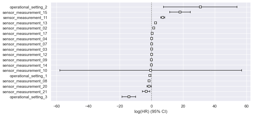
ctv.print_summary()
plt.figure(figsize=(10,5))
ctv.plot()
plt.show()
plt.close()
| model | lifelines.CoxTimeVaryingFitter |
|---|---|
| event col | 'status' |
| number of subjects | 260 |
| number of periods | 53759 |
| number of events | 260 |
| partial log-likelihood | -525.48 |
| time fit was run | 2022-09-17 08:02:36 UTC |
| coef | exp(coef) | se(coef) | coef lower 95% | coef upper 95% | exp(coef) lower 95% | exp(coef) upper 95% | cmp to | z | p | -log2(p) | |
|---|---|---|---|---|---|---|---|---|---|---|---|
| operational_setting_1 | -1.02 | 0.36 | 0.22 | -1.45 | -0.58 | 0.23 | 0.56 | 0.00 | -4.58 | <0.005 | 17.71 |
| operational_setting_2 | 30.86 | 2.51e+13 | 11.87 | 7.59 | 54.12 | 1988.10 | 3.18e+23 | 0.00 | 2.60 | 0.01 | 6.74 |
| operational_setting_3 | -14.26 | 0.00 | 2.21 | -18.59 | -9.92 | 0.00 | 0.00 | 0.00 | -6.44 | <0.005 | 32.97 |
| sensor_measurement_02 | 1.50 | 4.49 | 0.25 | 1.01 | 1.99 | 2.76 | 7.31 | 0.00 | 6.04 | <0.005 | 29.31 |
| sensor_measurement_03 | 0.09 | 1.10 | 0.02 | 0.06 | 0.13 | 1.06 | 1.14 | 0.00 | 5.30 | <0.005 | 23.00 |
| sensor_measurement_04 | 0.11 | 1.11 | 0.02 | 0.07 | 0.14 | 1.08 | 1.15 | 0.00 | 6.38 | <0.005 | 32.36 |
| sensor_measurement_07 | 0.11 | 1.11 | 0.14 | -0.17 | 0.38 | 0.85 | 1.46 | 0.00 | 0.77 | 0.44 | 1.18 |
| sensor_measurement_08 | -1.42 | 0.24 | 0.14 | -1.69 | -1.15 | 0.18 | 0.32 | 0.00 | -10.32 | <0.005 | 80.56 |
| sensor_measurement_09 | 0.03 | 1.03 | 0.01 | 0.00 | 0.06 | 1.00 | 1.06 | 0.00 | 2.10 | 0.04 | 4.80 |
| sensor_measurement_10 | -0.45 | 0.64 | 29.28 | -57.83 | 56.94 | 0.00 | 5.34e+24 | 0.00 | -0.02 | 0.99 | 0.02 |
| sensor_measurement_11 | 7.20 | 1344.92 | 0.66 | 5.91 | 8.50 | 367.50 | 4921.91 | 0.00 | 10.88 | <0.005 | 89.22 |
| sensor_measurement_12 | 0.06 | 1.07 | 0.15 | -0.23 | 0.36 | 0.79 | 1.44 | 0.00 | 0.42 | 0.67 | 0.57 |
| sensor_measurement_13 | 2.61 | 13.62 | 0.28 | 2.07 | 3.16 | 7.91 | 23.46 | 0.00 | 9.41 | <0.005 | 67.49 |
| sensor_measurement_14 | -0.04 | 0.96 | 0.02 | -0.07 | -0.01 | 0.93 | 0.99 | 0.00 | -2.65 | 0.01 | 6.97 |
| sensor_measurement_15 | 18.04 | 6.82e+07 | 3.31 | 11.55 | 24.52 | 1.04e+05 | 4.46e+10 | 0.00 | 5.45 | <0.005 | 24.27 |
| sensor_measurement_17 | 0.40 | 1.50 | 0.07 | 0.26 | 0.54 | 1.30 | 1.72 | 0.00 | 5.62 | <0.005 | 25.66 |
| sensor_measurement_20 | -1.43 | 0.24 | 0.70 | -2.80 | -0.05 | 0.06 | 0.95 | 0.00 | -2.04 | 0.04 | 4.59 |
| sensor_measurement_21 | -3.36 | 0.03 | 1.19 | -5.69 | -1.04 | 0.00 | 0.35 | 0.00 | -2.84 | <0.005 | 7.77 |
<div>
| Partial AIC | 1086.96 |
|---|---|
| log-likelihood ratio test | 1328.00 on 18 df |
| -log2(p) of ll-ratio test | 898.23 |
</div>
Predict And Evaluate
RUL_timevary_df_rcensored = RUL_timevary_df[['machine_name', 'cycle', 'operational_setting_1',
       'operational_setting_2', 'operational_setting_3',
        'sensor_measurement_02',
       'sensor_measurement_03', 'sensor_measurement_04',

       'sensor_measurement_07', 'sensor_measurement_08',
       'sensor_measurement_09', 'sensor_measurement_10',
       'sensor_measurement_11', 'sensor_measurement_12',
       'sensor_measurement_13', 'sensor_measurement_14',
       'sensor_measurement_15',
       'sensor_measurement_17',  'sensor_measurement_20',
       'sensor_measurement_21', 'start', 'status', "RUL"]].copy()[RUL_timevary_df['cycle'] <= 215]

RUL_timevary_df_rcensored
| machine_name | cycle | operational_setting_1 | operational_setting_2 | operational_setting_3 | sensor_measurement_02 | sensor_measurement_03 | sensor_measurement_04 | sensor_measurement_07 | sensor_measurement_08 | ... | sensor_measurement_12 | sensor_measurement_13 | sensor_measurement_14 | sensor_measurement_15 | sensor_measurement_17 | sensor_measurement_20 | sensor_measurement_21 | start | status | RUL | |
|---|---|---|---|---|---|---|---|---|---|---|---|---|---|---|---|---|---|---|---|---|---|
| 0 | 1 | 1 | 34.9983 | 0.8400 | 100.0 | 555.32 | 1358.61 | 1137.23 | 194.64 | 2222.65 | ... | 183.06 | 2387.72 | 8048.56 | 9.3461 | 334 | 14.73 | 8.8071 | 0 | False | 148 |
| 1 | 1 | 2 | 41.9982 | 0.8408 | 100.0 | 549.90 | 1353.22 | 1125.78 | 138.51 | 2211.57 | ... | 130.42 | 2387.66 | 8072.30 | 9.3774 | 330 | 10.41 | 6.2665 | 1 | False | 147 |
| 2 | 1 | 3 | 24.9988 | 0.6218 | 60.0 | 537.31 | 1256.76 | 1047.45 | 175.71 | 1915.11 | ... | 164.22 | 2028.03 | 7864.87 | 10.8941 | 309 | 14.08 | 8.6723 | 2 | False | 146 |
| 3 | 1 | 4 | 42.0077 | 0.8416 | 100.0 | 549.51 | 1354.03 | 1126.38 | 138.46 | 2211.58 | ... | 130.72 | 2387.61 | 8068.66 | 9.3528 | 329 | 10.59 | 6.4701 | 3 | False | 145 |
| 4 | 1 | 5 | 25.0005 | 0.6203 | 60.0 | 537.07 | 1257.71 | 1047.93 | 175.05 | 1915.10 | ... | 164.31 | 2028.00 | 7861.23 | 10.8963 | 309 | 14.13 | 8.5286 | 4 | False | 144 |
| ... | ... | ... | ... | ... | ... | ... | ... | ... | ... | ... | ... | ... | ... | ... | ... | ... | ... | ... | ... | ... | ... |
| 53653 | 260 | 211 | 9.9985 | 0.2500 | 100.0 | 604.58 | 1510.23 | 1308.38 | 394.46 | 2318.91 | ... | 371.71 | 2388.11 | 8145.03 | 8.6239 | 368 | 28.69 | 17.1938 | 210 | False | 105 |
| 53654 | 260 | 212 | 35.0062 | 0.8400 | 100.0 | 555.67 | 1366.07 | 1132.65 | 194.45 | 2223.23 | ... | 183.63 | 2388.42 | 8083.57 | 9.2709 | 335 | 14.82 | 8.8813 | 211 | False | 104 |
| 53655 | 260 | 213 | 42.0066 | 0.8404 | 100.0 | 549.48 | 1353.35 | 1123.50 | 138.63 | 2212.20 | ... | 130.71 | 2388.38 | 8101.10 | 9.3430 | 331 | 10.65 | 6.3974 | 212 | False | 103 |
| 53656 | 260 | 214 | 0.0026 | 0.0001 | 100.0 | 643.07 | 1595.53 | 1409.50 | 554.03 | 2388.08 | ... | 521.82 | 2388.08 | 8159.58 | 8.4068 | 394 | 38.76 | 23.2706 | 213 | False | 102 |
| 53657 | 260 | 215 | 34.9994 | 0.8400 | 100.0 | 555.75 | 1363.27 | 1132.58 | 194.05 | 2223.26 | ... | 183.14 | 2388.43 | 8088.93 | 9.3100 | 335 | 14.90 | 8.8744 | 214 | False | 101 |
49862 rows × 23 columns
preds_df = RUL_timevary_df_rcensored.groupby("machine_name").last()
preds_df = preds_df[preds_df.status == False].copy()

preds_df_wo_RUL = preds_df.drop(['RUL'], axis=1)
predictions = pd.DataFrame(ctv.predict_log_partial_hazard(preds_df_wo_RUL), columns=['predictions'])
predictions.index = preds_df.index

predictions['RUL'] = preds_df['RUL']
predictions.head(10)
| predictions | RUL | |
|---|---|---|
| machine_name | ||
| 2 | 4.822688 | 54 |
| 4 | 7.431523 | 20 |
| 11 | -0.342774 | 56 |
| 12 | 3.713341 | 34 |
| 13 | 7.702615 | 12 |
| 31 | -2.501934 | 128 |
| 32 | 6.108181 | 66 |
| 41 | 4.688602 | 47 |
| 42 | 11.195667 | 6 |
| 47 | 5.124843 | 31 |
# plt.xlabel callable bugfix
import matplotlib.pyplot as plt
from importlib import reload
plt=reload(plt)

plt.figure(figsize=(15,5))
plt.plot(predictions['RUL'], predictions['predictions'], '.b')
xlim = plt.gca().get_xlim()
plt.xlim(xlim[1], xlim[0])
plt.xlabel('RUL')
plt.ylabel('log_partial_hazard')
plt.title('log_partial_hazard vs. Remaining useful Lifetime of all engines still working after cycle 215')
plt.show()
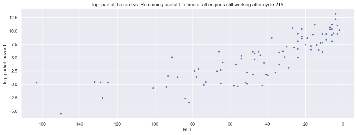
Predicting partial hazards
partial_hazard_df = RUL_timevary_df[['machine_name', 'cycle',
       'operational_setting_2', 'operational_setting_3',
        'sensor_measurement_02',
       'sensor_measurement_03', 'sensor_measurement_04',
       'sensor_measurement_07', 'sensor_measurement_08',
       'sensor_measurement_09', 'sensor_measurement_10',
       'sensor_measurement_11', 'sensor_measurement_12',
       'sensor_measurement_13', 'sensor_measurement_14',
       'sensor_measurement_15',
       'sensor_measurement_17',  'sensor_measurement_20',
       'sensor_measurement_21',  'start', 'status', "RUL"]].copy()

partial_hazard_df_test = RUL_timevary_df_test[['machine_name', 'cycle',
       'operational_setting_2', 'operational_setting_3',
        'sensor_measurement_02',
       'sensor_measurement_03', 'sensor_measurement_04',
       'sensor_measurement_07', 'sensor_measurement_08',
       'sensor_measurement_09', 'sensor_measurement_10',
       'sensor_measurement_11', 'sensor_measurement_12',
       'sensor_measurement_13', 'sensor_measurement_14',
       'sensor_measurement_15',
       'sensor_measurement_17',  'sensor_measurement_20',
       'sensor_measurement_21',  'start', 'status', "RUL"]].copy()

partial_hazard_df_wo_RUL =  partial_hazard_df.drop(['RUL'], axis=1)
partial_hazard_df_test_wo_RUL =  partial_hazard_df_test.drop(['RUL'], axis=1)
partial_hazard_df_wo_RUL.info()
<class 'pandas.core.frame.DataFrame'>
Int64Index: 53759 entries, 0 to 53758
Data columns (total 21 columns):
 #   Column                 Non-Null Count  Dtype
---  ------                 --------------  -----
 0   machine_name           53759 non-null  int64
 1   cycle                  53759 non-null  int64
 2   operational_setting_2  53759 non-null  float64
 3   operational_setting_3  53759 non-null  float64
 4   sensor_measurement_02  53759 non-null  float64
 5   sensor_measurement_03  53759 non-null  float64
 6   sensor_measurement_04  53759 non-null  float64
 7   sensor_measurement_07  53759 non-null  float64
 8   sensor_measurement_08  53759 non-null  float64
 9   sensor_measurement_09  53759 non-null  float64
 10  sensor_measurement_10  53759 non-null  float64
 11  sensor_measurement_11  53759 non-null  float64
 12  sensor_measurement_12  53759 non-null  float64
 13  sensor_measurement_13  53759 non-null  float64
 14  sensor_measurement_14  53759 non-null  float64
 15  sensor_measurement_15  53759 non-null  float64
 16  sensor_measurement_17  53759 non-null  int64
 17  sensor_measurement_20  53759 non-null  float64
 18  sensor_measurement_21  53759 non-null  float64
 19  start                  53759 non-null  int64
 20  status                 53759 non-null  bool
dtypes: bool(1), float64(16), int64(4)
memory usage: 8.7 MB
ctv_all = CoxTimeVaryingFitter()
ctv_all.fit(partial_hazard_df_wo_RUL, id_col="machine_name", event_col='status',
        start_col='start', stop_col='cycle', show_progress=True, step_size=1)
Iteration 45: norm_delta = 0.00315, step_size = 1.00000, ll = -537.06675, newton_decrement = 0.00000, seconds_since_start = 2.8Convergence completed after 45 iterations.


<lifelines.CoxTimeVaryingFitter: fitted with 53759 periods, 260 subjects, 260 events>
partial_hazard_df['log_partial_hazard'] = ctv_all.predict_log_partial_hazard(partial_hazard_df_wo_RUL)
partial_hazard_df_test['log_partial_hazard'] = ctv_all.predict_log_partial_hazard(partial_hazard_df_test_wo_RUL)
partial_hazard_df[-220:-1]
| machine_name | cycle | operational_setting_2 | operational_setting_3 | sensor_measurement_02 | sensor_measurement_03 | sensor_measurement_04 | sensor_measurement_07 | sensor_measurement_08 | sensor_measurement_09 | ... | sensor_measurement_13 | sensor_measurement_14 | sensor_measurement_15 | sensor_measurement_17 | sensor_measurement_20 | sensor_measurement_21 | start | status | RUL | log_partial_hazard | |
|---|---|---|---|---|---|---|---|---|---|---|---|---|---|---|---|---|---|---|---|---|---|
| 53539 | 260 | 97 | 0.6200 | 60.0 | 537.22 | 1255.25 | 1046.52 | 176.24 | 1915.32 | 8008.15 | ... | 2028.26 | 7874.49 | 10.8557 | 306 | 14.42 | 8.5486 | 96 | False | 219 | -2.405619 |
| 53540 | 260 | 98 | 0.0006 | 100.0 | 642.20 | 1586.33 | 1395.17 | 553.74 | 2388.05 | 9058.69 | ... | 2388.10 | 8135.97 | 8.3956 | 392 | 38.94 | 23.4231 | 97 | False | 218 | -7.915739 |
| 53541 | 260 | 99 | 0.0020 | 100.0 | 642.39 | 1593.33 | 1400.30 | 554.78 | 2388.07 | 9054.35 | ... | 2388.07 | 8137.09 | 8.4222 | 392 | 38.97 | 23.3577 | 98 | False | 217 | -5.113721 |
| 53542 | 260 | 100 | 0.8400 | 100.0 | 549.40 | 1355.57 | 1124.39 | 138.06 | 2211.87 | 8325.03 | ... | 2388.03 | 8088.60 | 9.3724 | 330 | 10.72 | 6.3828 | 99 | False | 216 | -2.618363 |
| 53543 | 260 | 101 | 0.6200 | 60.0 | 536.92 | 1262.05 | 1042.80 | 175.73 | 1915.34 | 8010.41 | ... | 2028.23 | 7873.90 | 10.8736 | 307 | 14.17 | 8.5988 | 100 | False | 215 | -1.891851 |
| ... | ... | ... | ... | ... | ... | ... | ... | ... | ... | ... | ... | ... | ... | ... | ... | ... | ... | ... | ... | ... | ... |
| 53753 | 260 | 311 | 0.0010 | 100.0 | 644.15 | 1604.81 | 1427.53 | 552.02 | 2388.13 | 9184.23 | ... | 2388.14 | 8246.20 | 8.5303 | 396 | 38.46 | 23.1252 | 310 | False | 5 | 11.023303 |
| 53754 | 260 | 312 | 0.7000 | 100.0 | 608.79 | 1495.60 | 1269.51 | 334.00 | 2324.92 | 8852.27 | ... | 2389.02 | 8169.64 | 9.3035 | 369 | 24.36 | 14.5189 | 311 | False | 4 | 7.773097 |
| 53755 | 260 | 313 | 0.2510 | 100.0 | 605.81 | 1514.32 | 1324.12 | 392.46 | 2319.17 | 8915.86 | ... | 2388.42 | 8245.36 | 8.7586 | 374 | 28.10 | 16.9454 | 312 | False | 3 | 11.300359 |
| 53756 | 260 | 314 | 0.6200 | 60.0 | 537.48 | 1276.24 | 1057.92 | 175.11 | 1917.37 | 8114.33 | ... | 2030.33 | 7971.25 | 11.0657 | 310 | 14.19 | 8.5503 | 313 | False | 2 | 11.386472 |
| 53757 | 260 | 315 | 0.6220 | 60.0 | 537.84 | 1272.95 | 1066.30 | 174.81 | 1917.36 | 8112.63 | ... | 2030.35 | 7972.47 | 11.0537 | 311 | 14.05 | 8.3729 | 314 | False | 1 | 14.245753 |
219 rows × 23 columns
rul10ph = partial_hazard_df[partial_hazard_df.RUL < 11][['RUL', 'log_partial_hazard']]
rul10ph
| RUL | log_partial_hazard | |
|---|---|---|
| 138 | 10 | 9.825637 |
| 139 | 9 | 8.224007 |
| 140 | 8 | 10.549260 |
| 141 | 7 | 9.158902 |
| 142 | 6 | 7.731988 |
| ... | ... | ... |
| 53754 | 4 | 7.773097 |
| 53755 | 3 | 11.300359 |
| 53756 | 2 | 11.386472 |
| 53757 | 1 | 14.245753 |
| 53758 | 0 | 10.462597 |
2860 rows × 2 columns
# plt.xlabel callable bugfix
import matplotlib.pyplot as plt
from importlib import reload
plt=reload(plt)

sns.set(rc = {'figure.figsize':(16,6)})
plt.scatter(partial_hazard_df['RUL'], partial_hazard_df['log_partial_hazard'])

plt.ylabel('log_partial_hazard')
plt.xlabel('RUL')
plt.axhline(y=5,ls="--",c=".5")
xlim = plt.gca().get_xlim()
plt.xlim(xlim[1], xlim[0])
plt.title('Train data - RUL vs. log partial hazard')

plt.show()
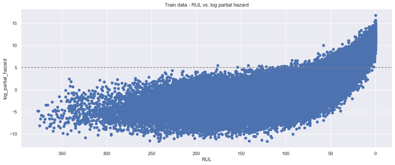
sns.set(rc = {'figure.figsize':(16,9)})
g = sns.FacetGrid(rul10ph, col="RUL",
                  #height=12,
                  #aspect=1.2,
                  col_wrap=4)
g.map(sns.histplot, "log_partial_hazard")
g.map(plt.axvline,x=10,ls="--",c=".5", color='r',)
plt.show()
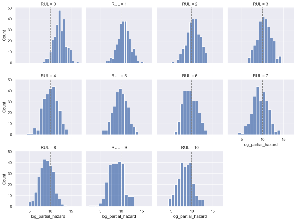
Simulate Engine Retirement Heuristic before RUL = 0
Training data
%%time
sns.set(rc = {'figure.figsize':(8,5)})

def loghaz_stopheuristic(df, threshold, recurrence_limit, method='consecutive', window=11):
    machinelist = df.machine_name.unique()
    decision_df = pd.DataFrame(index=machinelist)
    df['stop_decision'] = np.nan
    df['stop_decision_when'] = np.nan
    for m in machinelist:
        mask = (df.machine_name == m)
        temp = df[mask & (df.RUL < (window + 1))]
        overcount = 0
        for index, row in enumerate(temp.itertuples(), 1):
            if row.log_partial_hazard > threshold:
                 overcount += 1
            elif method=='consecutive':
                 overcount = 0
            if overcount > recurrence_limit:
                if row.RUL != 0:
                    decision_df.loc[m , 'stop_decision'] = True
                decision_df.loc[m , 'stop_decision_when'] = row.RUL
                #print(f'machine {m} was stopped' )
                break

    return df, decision_df


result, decisions = loghaz_stopheuristic(partial_hazard_df, threshold=5.5, recurrence_limit=5, method='consecutive', window=16)

print(f'stopped: {decisions.sum()} total: {decisions.shape[0]}')

print(f'\nmedian rul: {decisions.stop_decision_when.median()}')
decisions.stop_decision_when.plot(kind='box')
plt.ylabel('RUL')
plt.title('Distribution of engines retired with remaining RUL before failure (RUL = 0)')
plt.show()
decisions.stop_decision_when.plot(kind='hist', bins=35)
#plt.xlabel('RUL')
plt.title('Histogramm of engines retired with remaining RUL')
plt.show()
stopped: stop_decision            260
stop_decision_when    2415.0
dtype: object total: 260

median rul: 11.0
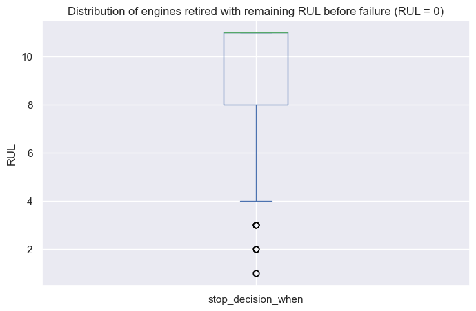
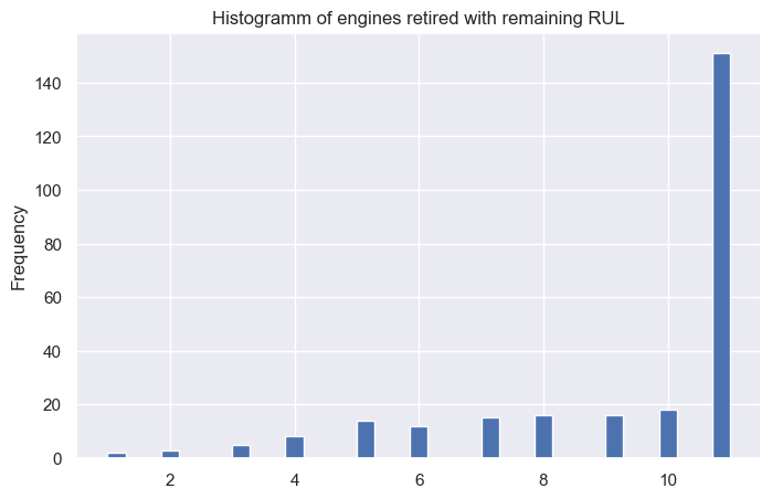
CPU times: total: 766 ms
Wall time: 761 ms
Verifiying with testing data
r, decisions_test = loghaz_stopheuristic(partial_hazard_df_test, threshold=5, recurrence_limit=3, method='consecutive', window=30)

print(f'stopped: {decisions_test.sum()} total: {decisions_test.shape[0]} median rul: {decisions_test.stop_decision_when.median()}')
decisions_test.stop_decision_when.plot(kind='box')
plt.ylabel('RUL')
plt.title('Distribution of engines retired with remaining RUL before failure (RUL = 0)')
plt.show()
decisions_test.stop_decision_when.plot(kind='hist', bins=35)
#plt.xlabel('RUL')
plt.title('Histogramm of engines retired with remaining RUL')
plt.show()
stopped: stop_decision            53
stop_decision_when    625.0
dtype: object total: 259 median rul: 10.0
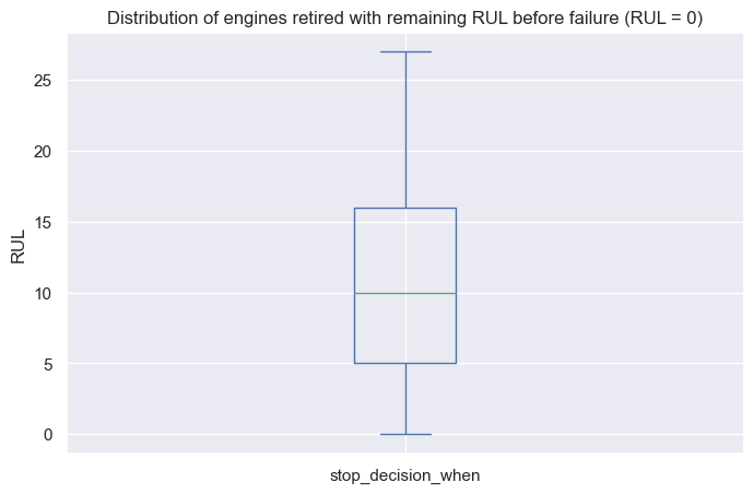
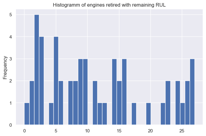
decisions_test
| stop_decision | stop_decision_when | |
|---|---|---|
| 1 | True | 27.0 |
| 2 | NaN | NaN |
| 3 | NaN | NaN |
| 4 | NaN | NaN |
| 5 | NaN | NaN |
| ... | ... | ... |
| 255 | NaN | NaN |
| 256 | NaN | NaN |
| 257 | NaN | NaN |
| 258 | NaN | NaN |
| 259 | NaN | NaN |
259 rows × 2 columns
# plt.xlabel callable bugfix
import matplotlib.pyplot as plt
from importlib import reload
plt=reload(plt)

sns.set(rc = {'figure.figsize':(16,11)})
plt.subplot(2,1,1)
#plt.figsize=(15,11)
plt.scatter(partial_hazard_df['RUL'], partial_hazard_df['log_partial_hazard'])

plt.ylabel('log_partial_hazard')
plt.xlabel('RUL')
plt.axhline(y=5,ls="--",c=".5")
xlim = plt.gca().get_xlim()
plt.xlim(xlim[1], xlim[0])
plt.title('Train data - RUL vs. log partial hazard')

plt.subplot(2,1,2)
plt.scatter(partial_hazard_df_test['RUL'], partial_hazard_df_test['log_partial_hazard'], color='g' )

xlim = plt.gca().get_xlim()
plt.xlim(xlim[1], xlim[0])

plt.ylabel('log_partial_hazard')
plt.xlabel('RUL')
plt.title('Test data - RUL vs. log partial hazard')
plt.show()
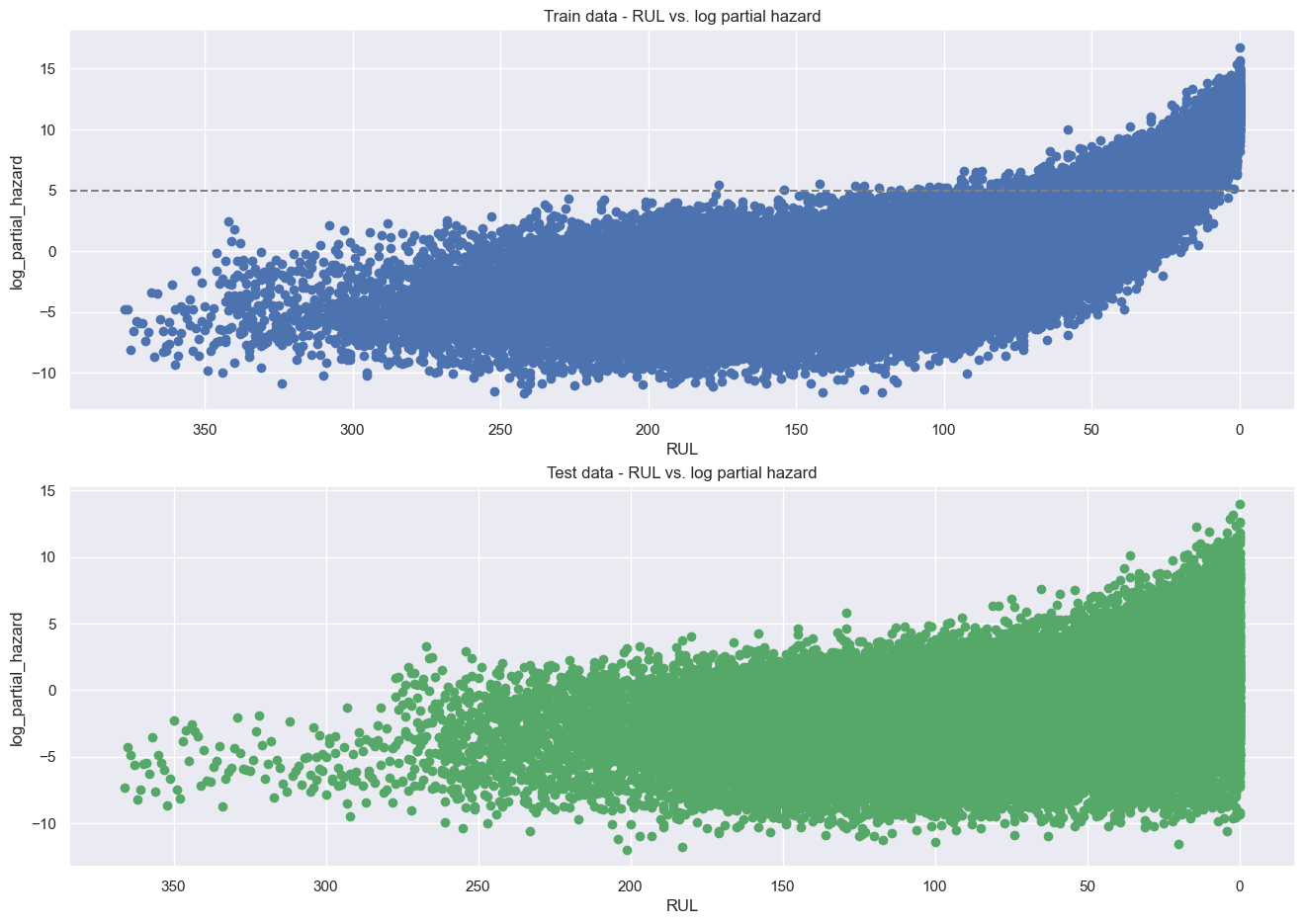
The CoxTimeVaryingFitted model was trained soley with training data of course. It performs well predicting log partial hazard values on the very same machines and is able to distinguish a nearing failure towards RUL=0 with virtually all log partial hazard values above a threshold of roundabout 5 pretty well from cycles that are far from end of RUL.
Predicting the same on the test data is however sobering as the model is seeing also elevated log partial hazard values it more often than not cannot distinguish near RUL zero engines from others. The model does not generalize well enough and is obviously overfitted. We have come to see the limitations of the CoxTimeVaryingFitting method as means of survival analysis and would recommend reapproach this problem with another algorithm and problem framing.
Update: Following up, I have reapproached this predictive maintenance problem again as a time series window classification problem, implemented as Long Short Term Memory (LSTM) type of recurrent neural network (RNN) suited for time series sequence data and its long-range dependencies. Please see here in my projects section: Predictive Maintenance ~ failure prediction with binary classification implemented as Gated Recurrent Units Recurrent Neural Network