Client Segments Data Simulation & Cost Sensitive Multi-classification
this notebook is loosely based on a given financial customer segmentation by BAI. https://www.latinia.com/IF/Documentos/The_New_Banking_Consumer_5_Core_Segments.pdf
Marketing research produces these kinds of segmentation through researching their market and collecting and mining a lot of data which is then used in their segmentation analysis, with clustering analysis, expert knowledge and loads of different quantitative and qualitative variables (predictors). This is what we cannot emulate here and instead accept as given.
The general goal of market segmentation is to find groups of customers that differ in important ways related to Product interest, market participation, or response to marketing efforts. By understanding the differences between groups, a marketer is enabled to take better strategic decisions about opportunities, product specification, the positioning, and engage in more effective advertising.
Finance segmentation
Banks and many other types of financial institutions classify their clients and try to perceive their behavioural structure which includes if they will pay their debts at all. If the bank has an improved understanding of the differences and nuances between these classes, then the bank can rethink of their marketing strategy. Resulting in more targeted, cost-effective approach and greater investment return.
Here is an example of banking customer segmentation by BAI Research Group.
Customer base is divided into 5 segments:
- Marginalised Middles
- Disengaged Skeptics
- Satisfied Traditionalists
- Struggling Techies
- Sophisticated Opportunists
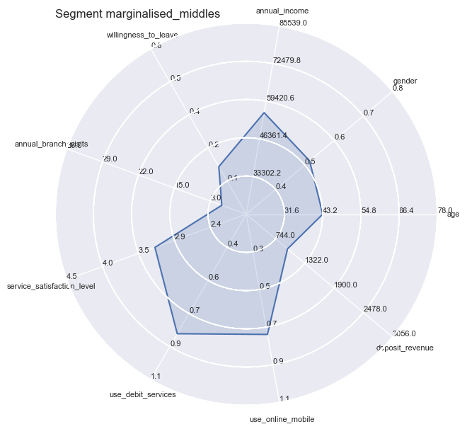
Marginalised Middles
It is the largest group containing 36% of the customers. This group is,
- Younger than the average age of 45.5
- Have larger annual income than average
- Least satisfied and most confused
- Least often visitor of the branches
- Most likely to pay someone else to handle their finances
Corresponding marketing strategy: Providing steady and clear marketing messages such as fee disclosure
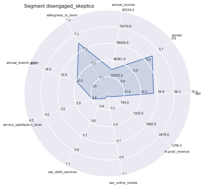
Disengaged Skeptics
It is the second oldest group of these 5. This group
- Earns below average
- Is the least satisfied with customer services
- Less likely to utilise available services like internet or mobile banking
- Has high concentration of accounts at other institutions
Corresponding marketing strategy: The door is open for other institutions to entice these unsatisfied group, be that other institution for this group.
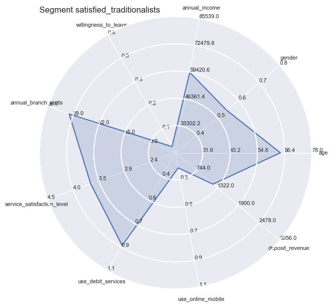
Satisfied Traditionalists
It is the oldest group with above average income. This segment:
- The least likely to use online, mobile, and debit services due to age and habits
- Has the second highest deposit revenue per household and expects a variety of product offerings
Corresponding marketing strategy: As this is a tempting segment with high deposit revenue and highest investment balance, offer them a wide product base.
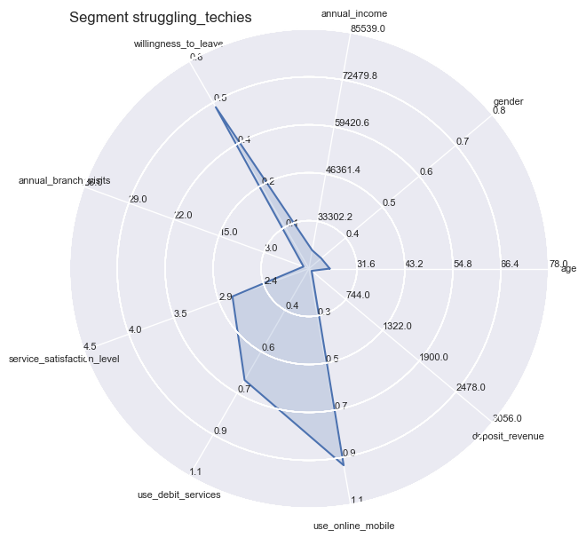
Struggling Techies
It is the youngest group with lowest income. Simply the youth and the youth has the features such as:
- Active in their finance
- Comfortable to make decisions
- Very receptive to other financial institutions with tempting offers
- Most likely to utilise online, mobile, and debit platforms
Corresponding marketing strategy: The receptivity of this segment makes them a worthwhile target. Easiest segment to gain new customers.
Sophisticated Opportunists
It has the average age and the highest income. This segment is
- The most satisfied with their primary financial institution
- Very knowledgeable about banking system and finance
- Has the highest return on mobile and debit services
- Has the highest deposit revenue per household
Corresponding marketing strategy: Treat this segment well, provide them with right tools and innovate products to allow them manage their own finance.
Source: https://www.segmentify.com/blog/customer-consumer-user-segmentation-examples#Marginalised_Middles
Client Segments Data Simulation
In this notebook we opt to interpret the given client segmentation model and generate our own data based on our assumptions and a modest variety of features and limited knowledge about the differences of these segments; it is not supposed to be a full fletched broad data generation effort. For doing the actual segmentation as a step in marketing research there will be more variables needed in order to delimit each segment better and still there will be always clients fitting only marginally better to one cluster than another. With this exercise we simulate the whole process with our own generated data and see if the code works before any real potential private data is exposed to exploratory analysis or machine learning further down the pipeline.
We can manipulate the synthetic data, re-run analyses, and examine how the results change. This data simulation highlights a strength of Python: it is easy to simulate data with various Python functions. And we will see that our limited dataset will be reasonably well suited to predict unsegmented clients to one of these given segments.
Let’s get started!
import numpy as np
import pandas as pd

pd.set_option('display.max_rows', 500)
pd.set_option('display.max_columns', 500)
pd.set_option('display.width', 70)
Client Segment Data Definitions
segment_variables = [
                     'age',
                     'gender',
                     'annual_income',
                     'willingness_to_leave',
                     'annual_branch_visits',
                     'service_satisfaction_level', # scale 1-5
                     'use_debit_services',
                     'use_online_mobile',
                     'deposit_revenue',

                     #'knowledgeable'

                    ]
segment_variables_distribution = dict(zip(segment_variables,
                                          [
                                            'normal',
                                           'binomial',
                                           'normal',
                                           'binomial',
                                           'poisson',
                                           'custom_discrete',
                                           'binomial',
                                           'binomial',
                                           #'binomial',
                                           'normal',

                                           #'binomial'
                                          ]
                                           ))

segment_variables_distribution['age']
'normal'
segment_variables_distribution
{'age': 'normal',
 'gender': 'binomial',
 'annual_income': 'normal',
 'willingness_to_leave': 'binomial',
 'annual_branch_visits': 'poisson',
 'service_satisfaction_level': 'custom_discrete',
 'use_debit_services': 'binomial',
 'use_online_mobile': 'binomial',
 'deposit_revenue': 'normal'}
segment_means = {'marginalised_middles':        [43, 0.45, 55000, 0.2, 6, None, 0.8, 0.7, 1000],
                 'disengaged_skeptics':         [54, 0.6, 38000, 0.5, 14, None, 0.2, 0.2, 340],
                 'satisfied_traditionalists':   [64, 0.55, 59000, 0.05, 30, None, 0.9, 0.15, 1200],
                 'struggling_techies':          [25, 0.45, 25000, 0.4, 2, None, 0.7, 0.9, 200],
                 'sophisticated_opportunists':  [45.5, 0.4, 70000, 0.2, 11, None, 0.9, 0.7, 2400]}
# standard deviations for each segment where applicable

segment_stddev = {'marginalised_middles':        [7, None, 10000, None, None, None, None, None,300],
                  'disengaged_skeptics':         [12, None, 7000, None, None, None, None, None, 120],
                  'satisfied_traditionalists':   [8, None, 11000, None, None, None, None, None,400],
                  'struggling_techies':          [4, None, 6000, None, None, None, None, None,80],
                  'sophisticated_opportunists':  [8, None, 16000, None, None, None, None, None,1000]}

# discrete variable probabilities
segment_pdist  = {'marginalised_middles':        [None, None, None, None, None,(0.05, 0.20, 0.35, 0.25, 0.15),None, None, None],
                  'disengaged_skeptics':         [None, None, None, None, None,(0.25, 0.25, 0.30, 0.15, 0.05),None, None, None],
                  'satisfied_traditionalists':   [None, None, None, None, None,(0.05, 0.10, 0.25, 0.30, 0.30),None, None, None],
                  'struggling_techies':          [None, None, None, None, None,(0.15, 0.25, 0.35, 0.20, 0.05),None, None, None],
                  'sophisticated_opportunists':  [None, None, None, None, None,(0.05, 0.15, 0.30, 0.25, 0.25),None, None, None]
                 }
segment_names = ['marginalised_middles', 'disengaged_skeptics', 'satisfied_traditionalists', 'struggling_techies',
                 'sophisticated_opportunists']
segment_sizes = dict(zip(segment_names,[180, 60, 160, 60, 40]))

segment_statistics = {}
for name in segment_names:
  segment_statistics[name] = {'size': segment_sizes[name]}
  for i, variable in enumerate(segment_variables):
    segment_statistics[name][variable] = {
        'mean': segment_means[name][i],
        'stddev': segment_stddev[name][i],
        'pdist': segment_pdist[name][i]
    }
Final segment data generation
#np.random.seed(seed=0)
from numpy.random import default_rng
from numpy.random import Generator, PCG64
from scipy import stats
rng = default_rng(0)
#rg = Generator(PCG64())
segment_constructor = {}

# Iterate over segments to create data for each
for name in segment_names:
  segment_data_subset = {}
  print('segment: {0}'.format(name))
  # Within each segment, iterate over the variables and generate data
  for variable in segment_variables:
    #print('\tvariable: {0}'.format(variable))
    if segment_variables_distribution[variable] == 'normal':

      #print(segment_statistics[name][variable]['mean'], segment_statistics[name][variable]['stddev'],segment_statistics[name]['size'] )
        # Draw random normals
      segment_data_subset[variable] = np.maximum(0, np.round(rng.normal(

          loc=segment_statistics[name][variable]['mean'],
          scale=segment_statistics[name][variable]['stddev'],
          size=segment_statistics[name]['size']

      ),2))
    elif segment_variables_distribution[variable] == 'poisson':
      # Draw counts
      segment_data_subset[variable] = rng.poisson(
          lam=segment_statistics[name][variable]['mean'],
          size=segment_statistics[name]['size']
      )
    elif segment_variables_distribution[variable] == 'binomial':
      # Draw binomials
      segment_data_subset[variable] = rng.binomial(
          n=1,
          p=segment_statistics[name][variable]['mean'],
          size=segment_statistics[name]['size']
      )
    elif segment_variables_distribution[variable] == 'custom_discrete':
      # Draw custom discrete ordinal variable
      xk = 1 + np.arange(5) # ordinal scale 1-5
      pk = segment_statistics[name][variable]['pdist']
      custm = stats.rv_discrete(name='custm', values=(xk, pk))
      segment_data_subset[variable] = custm.rvs(
          size=segment_statistics[name]['size']
      )
    else:
      # Data type unknown
      print('Bad segment data type: {0}'.format(
          segment_variables_distribution[j])
           )
      raise StopIteration
  segment_data_subset['Segment'] = np.repeat(
      name,
      repeats=segment_statistics[name]['size']
  )
  #print(segment_data_subset)

  segment_constructor[name] = pd.DataFrame(segment_data_subset)

segment_data = pd.concat(segment_constructor.values())
#segment_data.reindex(range(0,500,1))
segment_data.index = range(0,len(segment_data),1)
segment: marginalised_middles
segment: disengaged_skeptics
segment: satisfied_traditionalists
segment: struggling_techies
segment: sophisticated_opportunists
segment_data.index
RangeIndex(start=0, stop=500, step=1)
np.random.seed(seed=2554)
name = 'sophisticated_opportunists'
variable = 'age'
print(segment_statistics[name][variable]['mean'])
print(segment_statistics[name][variable]['stddev'])
np.random.normal(
    loc=segment_statistics[name][variable]['mean'],
    scale=segment_statistics[name][variable]['stddev'],
    size=10
)
45.5
8


array([51.99132515, 36.35474139, 53.75517472, 47.15209108, 48.3509104 ,
       47.01605492, 35.91508828, 67.32429057, 45.67072279, 36.21226966])
np.random.seed(seed=1)
variable = 'annual_branch_visits'
print(segment_statistics[name][variable]['mean'])
print(segment_statistics[name][variable]['stddev'])
np.random.poisson(
    lam=segment_statistics[name][variable]['mean'],
    size=10
)
11
None


array([10,  7,  7, 10, 10,  8, 10,  7,  9,  5])
np.random.seed(seed=2554)
variable = 'use_online_mobile'
print(segment_statistics[name][variable]['mean'])
print(segment_statistics[name][variable]['stddev'])
np.random.binomial(
    n=1,
    p=segment_statistics[name][variable]['mean'],
    size=10
)
0.7
None


array([0, 0, 1, 1, 1, 0, 0, 0, 1, 1])
np.repeat(name, repeats=10)
array(['sophisticated_opportunists', 'sophisticated_opportunists',
       'sophisticated_opportunists', 'sophisticated_opportunists',
       'sophisticated_opportunists', 'sophisticated_opportunists',
       'sophisticated_opportunists', 'sophisticated_opportunists',
       'sophisticated_opportunists', 'sophisticated_opportunists'],
      dtype='<U26')
# codings

segment_data['gender'] = segment_data['gender'].apply(
    lambda x: 'male' if x else 'female'
)
segment_data['use_online_mobile'] = segment_data['use_online_mobile'].apply(
    lambda x: True if x else False
)
segment_data['use_debit_services'] = segment_data['use_debit_services'].apply(
    lambda x: True if x else False
)
segment_data['willingness_to_leave'] = segment_data['willingness_to_leave'].apply(
    lambda x: True if x else False
)

# number adjustments
segment_data['service_satisfaction_level'] = segment_data['service_satisfaction_level'].apply(
    lambda x: np.minimum(x, 5)
)
segment_data.describe(include='all').T
| count | unique | top | freq | mean | std | min | 25% | 50% | 75% | max | |
|---|---|---|---|---|---|---|---|---|---|---|---|
| age | 500 | NaN | NaN | NaN | 49.1268 | 15.0625 | 14.31 | 38.9975 | 47.865 | 61.175 | 84.47 |
| gender | 500 | 2 | male | 258 | NaN | NaN | NaN | NaN | NaN | NaN | NaN |
| annual_income | 500 | NaN | NaN | NaN | 52407.5 | 16297.6 | 10933 | 42061.9 | 53450.3 | 63444.1 | 101433 |
| willingness_to_leave | 500 | 2 | False | 403 | NaN | NaN | NaN | NaN | NaN | NaN | NaN |
| annual_branch_visits | 500 | NaN | NaN | NaN | 14.568 | 11.8464 | 0 | 5 | 10 | 26 | 46 |
| service_satisfaction_level | 500 | NaN | NaN | NaN | 3.266 | 1.10711 | 1 | 3 | 3 | 4 | 5 |
| use_debit_services | 500 | 2 | True | 390 | NaN | NaN | NaN | NaN | NaN | NaN | NaN |
| use_online_mobile | 500 | 2 | True | 262 | NaN | NaN | NaN | NaN | NaN | NaN | NaN |
| deposit_revenue | 500 | NaN | NaN | NaN | 1008.83 | 710.295 | 0 | 471.582 | 939.565 | 1310.11 | 5545.03 |
| Segment | 500 | 5 | marginalised_middles | 180 | NaN | NaN | NaN | NaN | NaN | NaN | NaN |
Fortunately we can skip over the data cleaning part as we have generated a complete data set and almost ideal variables.
We may adjust a few columns where required.
Exploratory data analysis
the data we have just generated we have to understand, both predictors and Segments
| age | gender | annual_income | willingness_to_leave | annual_branch_visits | service_satisfaction_level | use_debit_services | use_online_mobile | deposit_revenue | Segment | |
|---|---|---|---|---|---|---|---|---|---|---|
| 0 | 43.88 | male | 54502.44 | True | 9 | 2 | True | True | 518.14 | marginalised_middles |
| 1 | 42.08 | male | 51325.97 | False | 5 | 3 | True | False | 1232.66 | marginalised_middles |
| 2 | 47.48 | female | 57187.86 | False | 9 | 5 | True | True | 841.21 | marginalised_middles |
| 3 | 43.73 | female | 63448.89 | False | 9 | 4 | True | True | 724.39 | marginalised_middles |
| 4 | 39.25 | male | 64933.36 | False | 6 | 3 | True | False | 668.41 | marginalised_middles |
# overview variable distributions by segment

segment_data.groupby('Segment').describe().T
| Segment | disengaged_skeptics | marginalised_middles | satisfied_traditionalists | sophisticated_opportunists | struggling_techies | |
|---|---|---|---|---|---|---|
| age | count | 60.000000 | 180.000000 | 160.000000 | 40.000000 | 60.000000 |
| mean | 51.970500 | 43.218778 | 64.607438 | 45.684000 | 25.020667 | |
| std | 11.292721 | 6.784148 | 9.112192 | 8.194710 | 4.466628 | |
| min | 26.240000 | 26.210000 | 41.360000 | 31.110000 | 14.310000 | |
| 25% | 44.340000 | 38.532500 | 59.020000 | 39.285000 | 22.070000 | |
| 50% | 52.685000 | 43.555000 | 65.175000 | 44.930000 | 25.465000 | |
| 75% | 58.415000 | 47.922500 | 70.787500 | 51.187500 | 28.087500 | |
| max | 75.350000 | 57.020000 | 84.470000 | 62.450000 | 35.590000 | |
| annual_income | count | 60.000000 | 180.000000 | 160.000000 | 40.000000 | 60.000000 |
| mean | 39231.491833 | 55453.384333 | 59366.816563 | 71282.635500 | 25304.253667 | |
| std | 7327.794135 | 10107.554102 | 11499.046189 | 15910.780974 | 5859.651345 | |
| min | 23278.540000 | 16005.780000 | 36366.400000 | 34845.970000 | 10933.040000 | |
| 25% | 34189.782500 | 48449.300000 | 51417.595000 | 59929.825000 | 22691.042500 | |
| 50% | 39342.710000 | 54961.765000 | 59105.985000 | 69765.445000 | 24905.780000 | |
| 75% | 44564.330000 | 62889.307500 | 66734.842500 | 81407.995000 | 29252.742500 | |
| max | 55407.350000 | 76188.030000 | 88451.780000 | 101432.840000 | 36739.460000 | |
| annual_branch_visits | count | 60.000000 | 180.000000 | 160.000000 | 40.000000 | 60.000000 |
| mean | 14.600000 | 5.766667 | 30.100000 | 11.075000 | 1.850000 | |
| std | 3.340557 | 2.521638 | 5.586597 | 3.173508 | 1.549467 | |
| min | 6.000000 | 1.000000 | 14.000000 | 5.000000 | 0.000000 | |
| 25% | 12.750000 | 4.000000 | 27.000000 | 8.750000 | 1.000000 | |
| 50% | 14.000000 | 6.000000 | 30.000000 | 12.000000 | 2.000000 | |
| 75% | 17.000000 | 7.000000 | 34.000000 | 13.000000 | 2.000000 | |
| max | 25.000000 | 14.000000 | 46.000000 | 17.000000 | 8.000000 | |
| service_satisfaction_level | count | 60.000000 | 180.000000 | 160.000000 | 40.000000 | 60.000000 |
| mean | 2.533333 | 3.188889 | 3.650000 | 3.500000 | 3.050000 | |
| std | 0.999435 | 1.066446 | 1.071060 | 0.847319 | 1.141290 | |
| min | 1.000000 | 1.000000 | 1.000000 | 2.000000 | 1.000000 | |
| 25% | 2.000000 | 2.000000 | 3.000000 | 3.000000 | 2.000000 | |
| 50% | 2.500000 | 3.000000 | 4.000000 | 4.000000 | 3.000000 | |
| 75% | 3.000000 | 4.000000 | 4.000000 | 4.000000 | 4.000000 | |
| max | 5.000000 | 5.000000 | 5.000000 | 5.000000 | 5.000000 | |
| deposit_revenue | count | 60.000000 | 180.000000 | 160.000000 | 40.000000 | 60.000000 |
| mean | 351.461667 | 981.358500 | 1202.073187 | 2546.885250 | 207.887000 | |
| std | 117.945737 | 285.727065 | 395.677513 | 1084.883418 | 79.367803 | |
| min | 100.540000 | 203.520000 | 158.100000 | 0.000000 | 36.660000 | |
| 25% | 269.722500 | 794.452500 | 925.917500 | 2089.477500 | 155.627500 | |
| 50% | 357.580000 | 957.185000 | 1178.785000 | 2513.155000 | 226.915000 | |
| 75% | 427.220000 | 1190.232500 | 1501.735000 | 2949.432500 | 255.882500 | |
| max | 661.050000 | 1713.780000 | 2405.490000 | 5545.030000 | 362.050000 |
import matplotlib.pyplot as plt
import seaborn as sns
sns.set_style("dark")
plt.figure(figsize=(10,7))

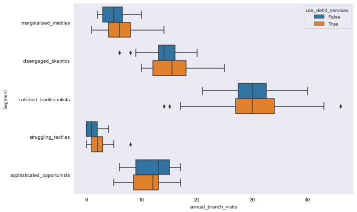
sns.boxplot(y='Segment', x='annual_branch_visits', hue='use_debit_services', data=segment_data,
             orient='h')
<AxesSubplot:xlabel='annual_branch_visits', ylabel='Segment'>
plt.figure(figsize=(10,7))
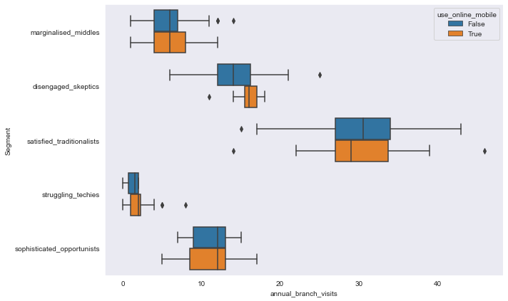
sns.boxplot(y='Segment', x='annual_branch_visits', hue='use_online_mobile', data=segment_data,
             orient='h')
<AxesSubplot:xlabel='annual_branch_visits', ylabel='Segment'>
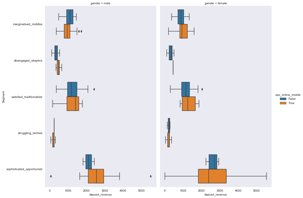
sns.catplot(y='Segment', x='deposit_revenue', hue='use_online_mobile', col="gender",
                data=segment_data, kind="box", height=9,
                aspect=.7);
plt.figure(figsize=(8,6))
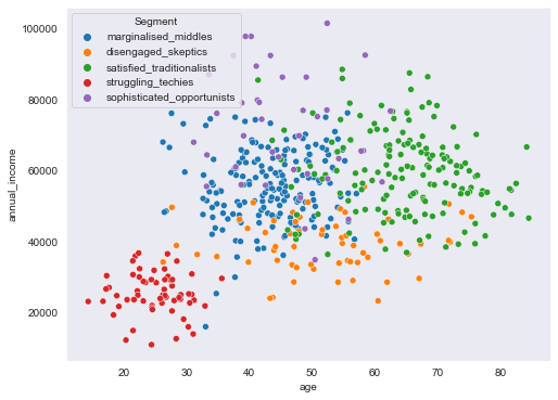
sns.scatterplot(data=segment_data, x="age", y="annual_income", hue=segment_data.Segment)
<AxesSubplot:xlabel='age', ylabel='annual_income'>
plt.figure(figsize=(8,6))
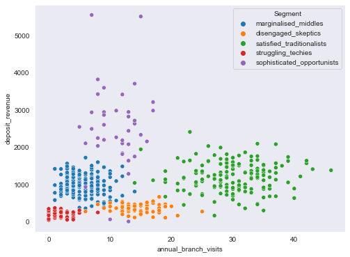
sns.scatterplot(data=segment_data, x="annual_branch_visits", y="deposit_revenue", hue=segment_data.Segment)
<AxesSubplot:xlabel='annual_branch_visits', ylabel='deposit_revenue'>
plt.figure(figsize=(8,6))
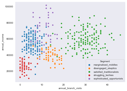
sns.scatterplot(data=segment_data, x="annual_branch_visits", y="annual_income", hue=segment_data.Segment)
<AxesSubplot:xlabel='annual_branch_visits', ylabel='annual_income'>
plt.figure(figsize=(8,6))
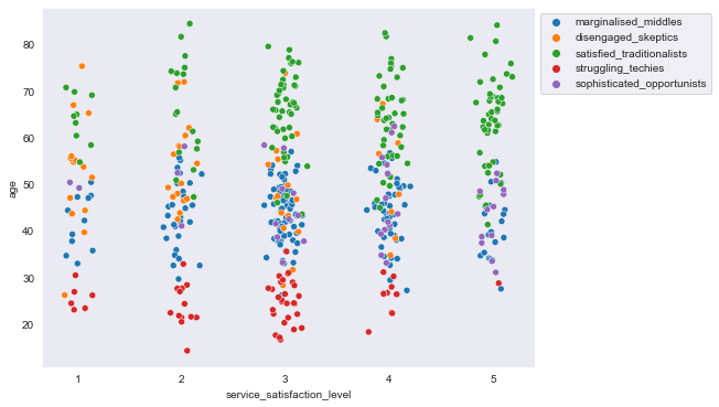
sns.scatterplot(data=segment_data, x=segment_data.service_satisfaction_level + np.random.normal(scale=0.08,
size=sum(segment_sizes.values())) , y="age", hue=segment_data.Segment)
plt.legend(bbox_to_anchor=(1,1), loc="upper left")
<matplotlib.legend.Legend at 0x18208f96cc0>
# create the main dataframe
#from sklearn import preprocessing
df = segment_data.copy()
df.describe(include='all').T
| count | unique | top | freq | mean | std | min | 25% | 50% | 75% | max | |
|---|---|---|---|---|---|---|---|---|---|---|---|
| age | 500 | NaN | NaN | NaN | 49.1268 | 15.0625 | 14.31 | 38.9975 | 47.865 | 61.175 | 84.47 |
| gender | 500 | 2 | male | 258 | NaN | NaN | NaN | NaN | NaN | NaN | NaN |
| annual_income | 500 | NaN | NaN | NaN | 52407.5 | 16297.6 | 10933 | 42061.9 | 53450.3 | 63444.1 | 101433 |
| willingness_to_leave | 500 | 2 | False | 403 | NaN | NaN | NaN | NaN | NaN | NaN | NaN |
| annual_branch_visits | 500 | NaN | NaN | NaN | 14.568 | 11.8464 | 0 | 5 | 10 | 26 | 46 |
| service_satisfaction_level | 500 | NaN | NaN | NaN | 3.242 | 1.1654 | 1 | 3 | 3 | 4 | 5 |
| use_debit_services | 500 | 2 | True | 390 | NaN | NaN | NaN | NaN | NaN | NaN | NaN |
| use_online_mobile | 500 | 2 | True | 262 | NaN | NaN | NaN | NaN | NaN | NaN | NaN |
| deposit_revenue | 500 | NaN | NaN | NaN | 1008.83 | 710.295 | 0 | 471.582 | 939.565 | 1310.11 | 5545.03 |
| Segment | 500 | 5 | marginalised_middles | 180 | NaN | NaN | NaN | NaN | NaN | NaN | NaN |
df.groupby('Segment').describe(include='all')
| age | gender | annual_income | willingness_to_leave | annual_branch_visits | service_satisfaction_level | use_debit_services | use_online_mobile | deposit_revenue | |||||||||||||||||||||||||||||||||||||||||||||||||||||||||||||||||||||||||||||||||||||||||||
|---|---|---|---|---|---|---|---|---|---|---|---|---|---|---|---|---|---|---|---|---|---|---|---|---|---|---|---|---|---|---|---|---|---|---|---|---|---|---|---|---|---|---|---|---|---|---|---|---|---|---|---|---|---|---|---|---|---|---|---|---|---|---|---|---|---|---|---|---|---|---|---|---|---|---|---|---|---|---|---|---|---|---|---|---|---|---|---|---|---|---|---|---|---|---|---|---|---|---|---|
| count | unique | top | freq | mean | std | min | 25% | 50% | 75% | max | count | unique | top | freq | mean | std | min | 25% | 50% | 75% | max | count | unique | top | freq | mean | std | min | 25% | 50% | 75% | max | count | unique | top | freq | mean | std | min | 25% | 50% | 75% | max | count | unique | top | freq | mean | std | min | 25% | 50% | 75% | max | count | unique | top | freq | mean | std | min | 25% | 50% | 75% | max | count | unique | top | freq | mean | std | min | 25% | 50% | 75% | max | count | unique | top | freq | mean | std | min | 25% | 50% | 75% | max | count | unique | top | freq | mean | std | min | 25% | 50% | 75% | max | |
| Segment | |||||||||||||||||||||||||||||||||||||||||||||||||||||||||||||||||||||||||||||||||||||||||||||||||||
| disengaged_skeptics | 60.0 | NaN | NaN | NaN | 51.970500 | 11.292721 | 26.24 | 44.3400 | 52.685 | 58.4150 | 75.35 | 60 | 2 | male | 39 | NaN | NaN | NaN | NaN | NaN | NaN | NaN | 60.0 | NaN | NaN | NaN | 39231.491833 | 7327.794135 | 23278.54 | 34189.7825 | 39342.710 | 44564.3300 | 55407.35 | 60 | 2 | False | 35 | NaN | NaN | NaN | NaN | NaN | NaN | NaN | 60.0 | NaN | NaN | NaN | 14.600000 | 3.340557 | 6.0 | 12.75 | 14.0 | 17.0 | 25.0 | 60.0 | NaN | NaN | NaN | 2.400000 | 1.092346 | 1.0 | 1.75 | 2.0 | 3.0 | 5.0 | 60 | 2 | False | 44 | NaN | NaN | NaN | NaN | NaN | NaN | NaN | 60 | 2 | False | 52 | NaN | NaN | NaN | NaN | NaN | NaN | NaN | 60.0 | NaN | NaN | NaN | 351.461667 | 117.945737 | 100.54 | 269.7225 | 357.580 | 427.2200 | 661.05 |
| marginalised_middles | 180.0 | NaN | NaN | NaN | 43.218778 | 6.784148 | 26.21 | 38.5325 | 43.555 | 47.9225 | 57.02 | 180 | 2 | male | 93 | NaN | NaN | NaN | NaN | NaN | NaN | NaN | 180.0 | NaN | NaN | NaN | 55453.384333 | 10107.554102 | 16005.78 | 48449.3000 | 54961.765 | 62889.3075 | 76188.03 | 180 | 2 | False | 149 | NaN | NaN | NaN | NaN | NaN | NaN | NaN | 180.0 | NaN | NaN | NaN | 5.766667 | 2.521638 | 1.0 | 4.00 | 6.0 | 7.0 | 14.0 | 180.0 | NaN | NaN | NaN | 3.222222 | 1.059965 | 1.0 | 3.00 | 3.0 | 4.0 | 5.0 | 180 | 2 | True | 153 | NaN | NaN | NaN | NaN | NaN | NaN | NaN | 180 | 2 | True | 133 | NaN | NaN | NaN | NaN | NaN | NaN | NaN | 180.0 | NaN | NaN | NaN | 981.358500 | 285.727065 | 203.52 | 794.4525 | 957.185 | 1190.2325 | 1713.78 |
| satisfied_traditionalists | 160.0 | NaN | NaN | NaN | 64.607438 | 9.112192 | 41.36 | 59.0200 | 65.175 | 70.7875 | 84.47 | 160 | 2 | male | 87 | NaN | NaN | NaN | NaN | NaN | NaN | NaN | 160.0 | NaN | NaN | NaN | 59366.816563 | 11499.046189 | 36366.40 | 51417.5950 | 59105.985 | 66734.8425 | 88451.78 | 160 | 2 | False | 155 | NaN | NaN | NaN | NaN | NaN | NaN | NaN | 160.0 | NaN | NaN | NaN | 30.100000 | 5.586597 | 14.0 | 27.00 | 30.0 | 34.0 | 46.0 | 160.0 | NaN | NaN | NaN | 3.625000 | 1.174948 | 1.0 | 3.00 | 4.0 | 5.0 | 5.0 | 160 | 2 | True | 145 | NaN | NaN | NaN | NaN | NaN | NaN | NaN | 160 | 2 | False | 126 | NaN | NaN | NaN | NaN | NaN | NaN | NaN | 160.0 | NaN | NaN | NaN | 1202.073187 | 395.677513 | 158.10 | 925.9175 | 1178.785 | 1501.7350 | 2405.49 |
| sophisticated_opportunists | 40.0 | NaN | NaN | NaN | 45.684000 | 8.194710 | 31.11 | 39.2850 | 44.930 | 51.1875 | 62.45 | 40 | 2 | female | 21 | NaN | NaN | NaN | NaN | NaN | NaN | NaN | 40.0 | NaN | NaN | NaN | 71282.635500 | 15910.780974 | 34845.97 | 59929.8250 | 69765.445 | 81407.9950 | 101432.84 | 40 | 2 | False | 32 | NaN | NaN | NaN | NaN | NaN | NaN | NaN | 40.0 | NaN | NaN | NaN | 11.075000 | 3.173508 | 5.0 | 8.75 | 12.0 | 13.0 | 17.0 | 40.0 | NaN | NaN | NaN | 3.750000 | 1.126601 | 1.0 | 3.00 | 4.0 | 5.0 | 5.0 | 40 | 2 | True | 35 | NaN | NaN | NaN | NaN | NaN | NaN | NaN | 40 | 2 | True | 31 | NaN | NaN | NaN | NaN | NaN | NaN | NaN | 40.0 | NaN | NaN | NaN | 2546.885250 | 1084.883418 | 0.00 | 2089.4775 | 2513.155 | 2949.4325 | 5545.03 |
| struggling_techies | 60.0 | NaN | NaN | NaN | 25.020667 | 4.466628 | 14.31 | 22.0700 | 25.465 | 28.0875 | 35.59 | 60 | 2 | female | 40 | NaN | NaN | NaN | NaN | NaN | NaN | NaN | 60.0 | NaN | NaN | NaN | 25304.253667 | 5859.651345 | 10933.04 | 22691.0425 | 24905.780 | 29252.7425 | 36739.46 | 60 | 2 | False | 32 | NaN | NaN | NaN | NaN | NaN | NaN | NaN | 60.0 | NaN | NaN | NaN | 1.850000 | 1.549467 | 0.0 | 1.00 | 2.0 | 2.0 | 8.0 | 60.0 | NaN | NaN | NaN | 2.783333 | 0.903696 | 1.0 | 2.00 | 3.0 | 3.0 | 5.0 | 60 | 2 | True | 41 | NaN | NaN | NaN | NaN | NaN | NaN | NaN | 60 | 2 | True | 56 | NaN | NaN | NaN | NaN | NaN | NaN | NaN | 60.0 | NaN | NaN | NaN | 207.887000 | 79.367803 | 36.66 | 155.6275 | 226.915 | 255.8825 | 362.05 |
print(segment_data.dtypes)
df.dtypes.value_counts()
age                           float64
gender                         object
annual_income                 float64
willingness_to_leave             bool
annual_branch_visits            int64
service_satisfaction_level      int64
use_debit_services               bool
use_online_mobile                bool
deposit_revenue               float64
Segment                        object
dtype: object


float64    3
bool       3
int64      2
object     2
dtype: int64
this dataset consists of mixed variable types, numeric such as float64 and int as well as categorical object type and boolean data.
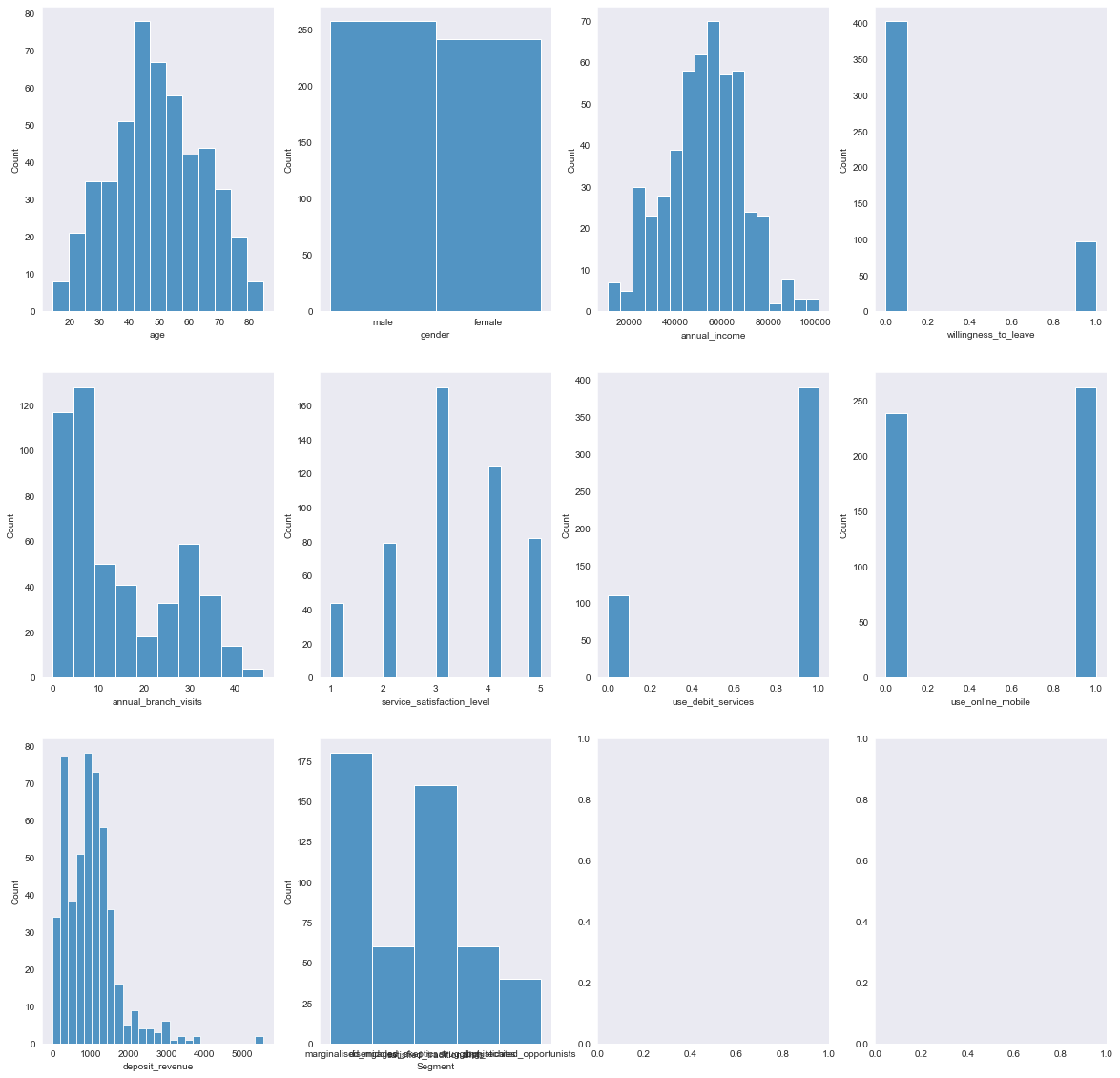
# frequencies plotted in Histogramms
import warnings
with warnings.catch_warnings():
    warnings.simplefilter('ignore')

f, axes = plt.subplots(3,4, figsize=(20, 20))
for ax, feature in zip(axes.flat, df.columns):
    sns.histplot(df[feature], ax=ax)
<string>:6: RuntimeWarning: Converting input from bool to <class 'numpy.uint8'> for compatibility.
<string>:6: RuntimeWarning: Converting input from bool to <class 'numpy.uint8'> for compatibility.
<string>:6: RuntimeWarning: Converting input from bool to <class 'numpy.uint8'> for compatibility.
<string>:6: RuntimeWarning: Converting input from bool to <class 'numpy.uint8'> for compatibility.
<string>:6: RuntimeWarning: Converting input from bool to <class 'numpy.uint8'> for compatibility.
<string>:6: RuntimeWarning: Converting input from bool to <class 'numpy.uint8'> for compatibility.
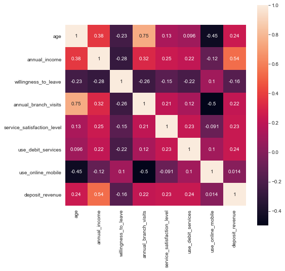
The standard in any explorative data analysis is the consultation of the correlations of the various features, due to the limitations to catch only linear relationships we do not spend too much time on this and rather turn to the Predictive Power Score.
# column pairwise correlations
plt.figure(figsize=(8,8))
sns.heatmap(df.corr('pearson'),annot = True, fmt='.2g', square=True)
<AxesSubplot:>
Predictive Power Score
Let’s use the Predictive Power Score (PPS) on this occasion to quickly unfold relations not only between predictors but also the Segment labels. The PPS is also directional, hence asymmetric, also can handle any data-type and can detect linear or non-linear relationships between two columns.
From the first row we can see at first sight the most influential predictors for the Segment as annual_branch_visits, age and deposit_revenue.
### ppscore package ###
import ppscore as pps
def heatmap(df):
    plt.rcParams['figure.figsize'] = (11,7)
    df = df[['x', 'y', 'ppscore']].pivot(columns='x', index='y', values='ppscore')
    ax = sns.heatmap(df, vmin=0, vmax=1, linewidths=0.5, annot=True)
    ax.set_title("PPS matrix")
    ax.set_xlabel("feature")
    ax.set_ylabel("target")
    return ax
def corr_heatmap(df):
    ax = sns.heatmap(df, vmin=-1, vmax=1, linewidths=0.5, annot=True)
    ax.set_title("Correlation matrix")
    return ax
### ppscore package ###

ppsmatrix = pps.matrix(df)
heatmap(ppsmatrix)
<AxesSubplot:title={'center':'PPS matrix'}, xlabel='feature', ylabel='target'>
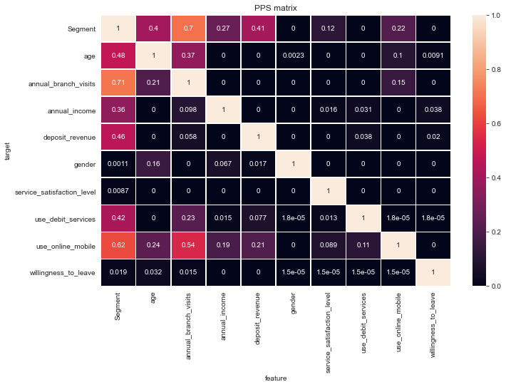
The PPS matrix is not symmetric like Pearsons correlations but can be read from feature to target or the other way round. So for instance we can learn from the matrix that we from the annual_branch_visits you can predict likelihood of online/mobile use with 0.54 quite moderately but much less so the reverse with only 0.15.
import seaborn as sns
sns.set(style="ticks", color_codes=True)
sns.set_style("dark")

plt.figure(figsize=(15,15))
customgrid = sns.pairplot(df, hue="Segment")
customgrid.map_upper(plt.scatter, linewidths=1, s=5, alpha=0.5)
plt.show()
<Figure size 1080x1080 with 0 Axes>
res = sns.relplot(data=df, x='annual_income', y='age', hue="Segment", alpha=0.6, col="use_online_mobile")
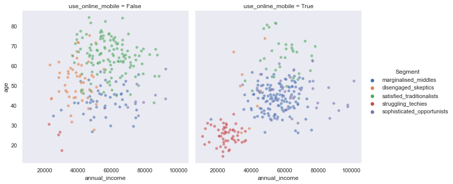
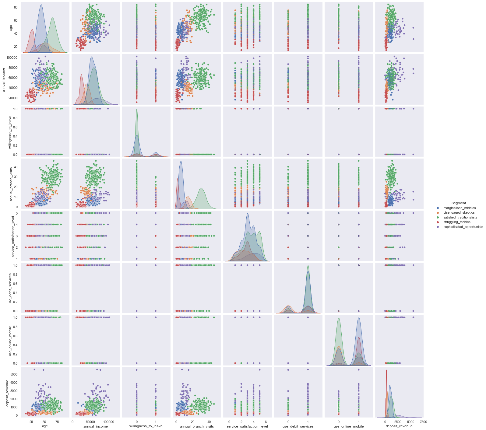
We could use Seaborn relational plots to observe multiple independent variables per Segment.
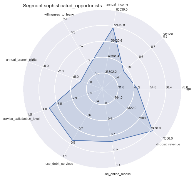
However you still could not apply all independent variables all at the same time, therefore we turn towards Radar Plots / Spider plots which are great for complete profiling as long as the number of variables are manageable or can be reduced to a handful of essentiell ones.
# https://gist.github.com/kylerbrown/29ce940165b22b8f25f4

import numpy as np
import matplotlib.pyplot as plt
import seaborn as sns # improves plot aesthetics
from textwrap import wrap
import matplotlib.patches as mpatches

def _invert(x, limits):
    """inverts a value x on a scale from
    limits[0] to limits[1]"""
    return limits[1] - (x - limits[0])

def _scale_data(data, ranges):
    """scales data[1:] to ranges[0],
    inverts if the scale is reversed"""
    for d, (y1, y2) in zip(data[1:], ranges[1:]):
        #print( d, (y1, y2))
        assert (y1 <= d <= y2) or (y2 <= d <= y1)
    x1, x2 = ranges[0]
    d = data[0]
    if x1 > x2:
        d = _invert(d, (x1, x2))
        x1, x2 = x2, x1
    sdata = [d]
    for d, (y1, y2) in zip(data[1:], ranges[1:]):
        if y1 > y2:
            d = _invert(d, (y1, y2))
            y1, y2 = y2, y1
        sdata.append((d-y1) / (y2-y1)
                     * (x2 - x1) + x1)
    return sdata

class ComplexRadar():
    def __init__(self, fig, variables, ranges,
                 n_ordinate_levels=6):
        angles = np.arange(0, 360, 360./len(variables))

        axes = [fig.add_axes([0.1,0.1,0.9,0.9],polar=True,
                label = "axes{}".format(i))
                for i in range(len(variables))]
        l, text = axes[0].set_thetagrids(angles,
                                         labels=variables)

        [txt.set_rotation(angle-90) for txt, angle
             in zip(text, angles)]

        for ax in axes[1:]:
            ax.patch.set_visible(False)
            ax.grid("off")
            ax.xaxis.set_visible(False)
        for i, ax in enumerate(axes):
            grid = np.linspace(*ranges[i],
                               num=n_ordinate_levels)
            gridlabel = ["{}".format(round(x,1))
                         for x in grid]
            if ranges[i][0] > ranges[i][1]:
                grid = grid[::-1] # hack to invert grid
                          # gridlabels aren't reversed
            gridlabel[0] = "" # clean up origin
            ax.set_rgrids(grid, labels=gridlabel,
                         angle=angles[i])
            #ax.spines["polar"].set_visible(False)
            ax.set_ylim(*ranges[i])
        # variables for plotting
        self.angle = np.deg2rad(np.r_[angles, angles[0]])
        self.ranges = ranges
        self.ax = axes[0]
    def plot(self, data, *args, **kw):
        sdata = _scale_data(data, self.ranges)
        r = self.ax.plot(self.angle, np.r_[sdata, sdata[0]], *args, **kw)
        return r
    def fill(self, data, *args, **kw):
        sdata = _scale_data(data, self.ranges)
        self.ax.fill(self.angle, np.r_[sdata, sdata[0]], *args, **kw)
    def legend(self, *args, **kw):
        self.ax.legend(self, *args, **kw)

# prepare data to be plotted in the segment profiles
criteria = ('age', 'gender', 'annual_income', 'willingness_to_leave',
       'annual_branch_visits', 'service_satisfaction_level',
       'use_debit_services',
            'use_online_mobile', 'deposit_revenue')

segmeans = df.copy()
segmeans['gender'] = segmeans['gender'].apply(lambda x: 1 if x == 'male' else 0)

segmeans['willingness_to_leave'] = segmeans['willingness_to_leave'].apply(lambda x: 1 if x == True else 0)
segmeans['use_debit_services'] = segmeans['use_debit_services'].apply(lambda x: 1 if x == True else 0)
segmeans['use_online_mobile'] = segmeans['use_online_mobile'].apply(lambda x: 1 if x == True else 0)

segmeans = segmeans.groupby('Segment').mean()

segs = df.Segment.unique()

#test = segdata.get('marginalised_middles')

data=[]
segdata = dict()

for seg in segs:
    #for crit in criteria:
    data.append(segmeans.loc[seg])

    segdata.update({seg: data})
    data = []

ranges = []
for col in segmeans.columns:
    #print(df[col].dtype)
    distance = 0.2 # increase in case of assert errors
    if segmeans[col].dtype != 'object' and segmeans[col].dtype != 'bool':
        lower = min(segmeans[col])- min(segmeans[col])* distance
        upper = max(segmeans[col])+ max(segmeans[col])* distance
        if upper > 10:
            upper = round(upper,0)
            lower = round(lower,0)
        else:
            upper = round(upper,1)
            lower = round(lower,1)
        ranges.append((lower,upper))

# plotting


plt.rc('xtick', labelsize=8)
plt.rc('ytick', labelsize=8)
i=0
for key, value in segdata.items():
    #print(key, value)
    #plt.title(key)
    radar = ComplexRadar(plt.figure(figsize=(6, 6), dpi = 100), criteria, ranges)
    radar.plot(tuple(value[0]))
    radar.fill(tuple(value[0]), alpha=0.2)
    #plt.tight_layout(pad=2)
    plt.title('Segment ' + str(key), loc='left')

plt.show()
import warnings
warnings.filterwarnings('ignore')
#ignore neglible user warning for legend params

comparisons = [['disengaged_skeptics', 'marginalised_middles'],
             ['satisfied_traditionalists', 'sophisticated_opportunists'],
             ['struggling_techies', 'disengaged_skeptics']]

for comparison in comparisons:
    segdatasliced = {key: segdata[key] for key in segdata.keys() & comparison}

    radar = ComplexRadar(plt.figure(figsize=(6, 6), dpi = 100), criteria, ranges)
    #init
    title = ''
    ha=[]
    la=[]
    for key, value in segdatasliced.items():
        r = radar.plot(tuple(value[0]))
        radar.fill(tuple(value[0]), alpha=0.2)

        patch = mpatches.Patch(color=r[0].get_color(), label=key)
        ha.append(patch)
        la.append(key)
        #radar.legend(, loc=1)
        #plt.tight_layout(pad=2)

        if len(title) > 1:
            title = 'Segment Means Profile Comparison: ' + title + ' vs. ' + key
        else:
            title = key

    radar.legend(handles=ha, labels=la, loc=1, bbox_to_anchor=(0.1, 0.1))
    plt.title('\n'.join(wrap(title,40)), loc='left',   x=-0.3, y=0.94, pad=14)
    plt.show()
Segment Means Profile comparisons
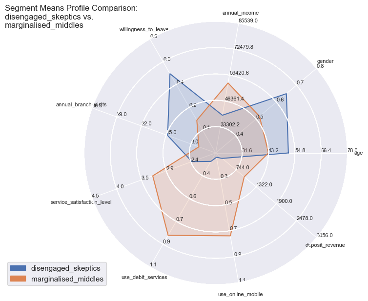
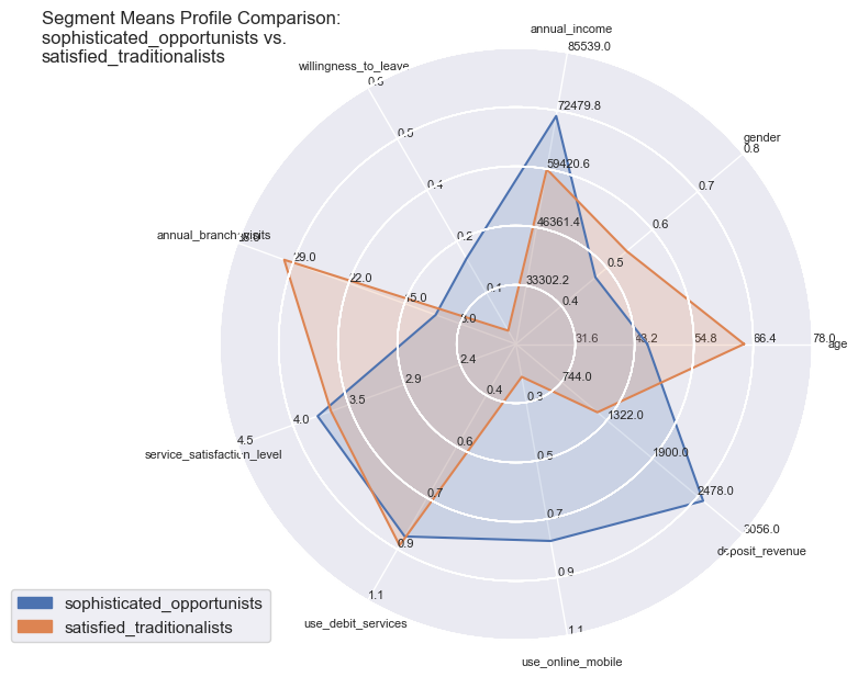
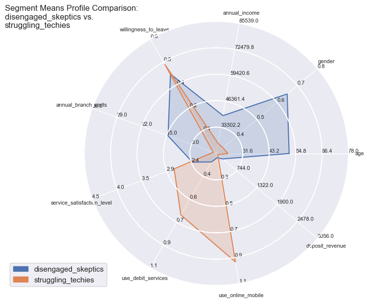
With radar plots the features average profiles can be visually compared to each other especially for those features which are particularly pronounced towards population max- and minima.
So the differences become quite apparent and could not be wider in certain combinations: whether it is the strong use of debit services of the ‘middles’ or the high willingness to leave of the ‘skeptics’. Both have in common the equally low service satisfaction rating on average.
Cost Sensitive Multi-classification
We assume we have a representative independent set of customer records which can be labeled by customer service and domain experts, we may able to create a classification model that can assign also every other customer record into the correct customer segment they belong to (Multi-class classification task). For this notebook we just use the above generated dataset.
Logistic regression model
So for such a classification I like to choose a Logistic Regression statistical model by default. With logistic regression there are a few assumptions to be met, before it can be applied and used.
Assumptions to be checked
- Appropriate outcome type - our case will be the multinomial regression where the dependent variable y will have more than two classes of outcomes.
- logistic regression requires the observations to be independent of each other. In other words, the observations should not come from repeated measurements or matched data.
- logistic regression requires there to be little or no multicollinearity among the independent variables. This means that the independent variables should not be too highly correlated with each other.
- logistic regression assumes linearity of independent variables and log odds. although this analysis does not require the dependent and independent variables to be related linearly, it requires that the independent variables are linearly related to the log odds.
- logistic regression typically requires a large sample size. A general guideline is that you need at minimum of 10 cases with the least frequent outcome for each independent variable in your model. For example, if you have 5 independent variables and the expected probability of your least frequent outcome is .10, then you would need a minimum sample size of 500 (10*5 / .10).
the first two assumptions can be checked off quickly: Firstly our case will be the multinomial regression where the dependent variable y will have more than two classes of outcomes, this is an appropiate type of outcome, so we check #1. Secondly all observations should be independent from each other, which is the case here too, as we have generated the data ourselves, we mark assumption number 2 as met as well.
checking assumption 3 - little or no multicollinearity of predictors
We will check all features for elevated mulicorrelation with the Variance Inflation Factor Check. We use the statsmodels package with the same name and prepare the data.
# looks like not needed anymore

"""df_test = df_unlabeled.copy()
df_test['Segment'] = segment_data.Segment
df_test.head()"""
"df_test = df_unlabeled.copy()\ndf_test['Segment'] = segment_data.Segment\ndf_test.head()"
"""import pandas as pd, numpy as np
from sklearn.preprocessing import MultiLabelBinarizer
import warnings
warnings.filterwarnings("ignore")

segm = df.copy()"""
'import pandas as pd, numpy as np\nfrom sklearn.preprocessing import MultiLabelBinarizer\nimport warnings\nwarnings.filterwarnings("ignore")\n\nsegm = df.copy()'
# copy as df
segm = df.copy()

segm['gender'] = segm['gender'].apply(
    lambda x: 1 if x == 'male' else 0
)
segm['use_online_mobile'] = segm['use_online_mobile'].apply(
    lambda x: 1 if x else 0
)
segm['use_debit_services'] = segm['use_debit_services'].apply(
    lambda x: 1 if x else 0
)
segm['willingness_to_leave'] = segm['willingness_to_leave'].apply(
    lambda x: 1 if x else 0
)

# copy as numpy array
segm_array = df.copy().values

X = segm_array[:, :segm.shape[1] - 1]
y = segm_array[:, segm.shape[1] - 1]
# Variance Inflation Factor Check for Multicollinearity

from statsmodels.stats.outliers_influence import variance_inflation_factor
from statsmodels.tools.tools import add_constant

df_vif = add_constant(segm.iloc[:,:-1])
pd.Series([variance_inflation_factor(df_vif.values, i) for i in range(df_vif.shape[1])], index=df_vif.columns)
const                         36.130813
age                            2.516610
gender                         1.023785
annual_income                  1.643256
willingness_to_leave           1.158922
annual_branch_visits           2.628614
service_satisfaction_level     1.152449
use_debit_services             1.168716
use_online_mobile              1.431586
deposit_revenue                1.490094
dtype: float64
The test shows light elevated factors for the variables ‘age’ and ‘annual_branch_visits’.
Levels around 1 are low, threshold to raise concerns range from 2.5 up to 10, and are therefore always subjective.
To be certain we use an other method to detect high-multi-collinearity by inspecting the eigen values of the correlation matrix.
A very low eigen value shows that the data are collinear, and the corresponding eigen vector could show which variables are then collinear. So put another way: if there is no collinearity in the data, you would expect that none of the eigen values are close to zero.
features = segm.iloc[:,:-1]

# correlation matrix
corr = np.corrcoef(features, rowvar=0)

# eigen values & eigen vectors
w, v = np.linalg.eig(corr)

# eigen vector of a predictor
# pd.Series(v[:,3], index=segm.iloc[:,:-1].columns)

pd.Series(w, index=features.columns)
age                           2.797363
gender                        1.526171
annual_income                 0.233061
willingness_to_leave          0.432331
annual_branch_visits          0.518614
service_satisfaction_level    0.704103
use_debit_services            1.032196
use_online_mobile             0.848536
deposit_revenue               0.907625
dtype: float64
The result shows that none of the eigen values could be rounded to zero one digit after the decimal point, so that is bascially enough to rule out a problem with multi-collinearity. We can tick assumption 3 as being checked as well.
Lets move quickly to assumption no 4 which requires linear relationships of the independent variables and the model’s log odds.
# Needed to run the logistic regression
import statsmodels.formula.api as smf

# For plotting/checking assumptions
import seaborn as sns

df_check = segm.copy()

df_check['gender'] = df['gender'].astype('category')
df_check['use_online_mobile'] = df['use_online_mobile'].astype('category')
df_check['use_debit_services'] = df['use_debit_services'].astype('category')
df_check['willingness_to_leave'] = df['willingness_to_leave'].astype('category')


mapdict = dict(zip( df_check.Segment.unique(), range(0,5)))
df_check['Segment'] = df_check.Segment.map(mapdict)

#df_check['Segment'] = df['Segment'].astype('category')
df_check = pd.get_dummies(df_check)
df_check.to_csv('df_check.csv', index=False)
#dummy_segs = df_check.iloc[:,-5:].columns
predictors = df_check.iloc[:,:9].columns
## sklearn
from sklearn.linear_model import LogisticRegression

# Logistic Regression
testmodel = LogisticRegression(multi_class='multinomial')
testmodel.fit(df_check.iloc[:,:-1], df_check['Segment'])

# only for the purpose of this assumption test we predict with training data
probabilities = testmodel.predict_proba(df_check.iloc[:,:-1])

logodds = pd.DataFrame(np.log(probabilities/(1-probabilities)))
logodds.head()
[0 1 2 3 4]
| 0 | 1 | 2 | 3 | 4 | |
|---|---|---|---|---|---|
| 0 | -0.332695 | -0.967721 | -1.193680 | -2.675036 | -4.593497 |
| 1 | -0.214611 | -4.825835 | -0.328147 | -13.571020 | -1.929562 |
| 2 | 0.123727 | -2.417282 | -0.575284 | -6.976273 | -3.611851 |
| 3 | 0.176263 | -1.583293 | -1.015212 | -4.618127 | -4.596909 |
| 4 | 0.152500 | -1.298140 | -1.288492 | -3.688953 | -4.958581 |
class_list = list(df.Segment.unique())
#yy = 10/pow(df_check.service_satisfaction_level + 3, 5)
#yy = df_check.service_satisfaction_level
yy = df_check.age
xx = logodds.iloc[:,4] # logodds for one class
from statsmodels.nonparametric.smoothers_lowess import lowess as  sm_lowess

plt.figure(figsize=(14,14))
plt.title('predictor age')

cols = 2
rows = np.ceil(len(df.Segment.unique()) / cols)

for i in range(0,len(df.Segment.unique())):
    ax = plt.subplot(rows, cols, i + 1)
    sm_y, sm_x = sm_lowess(yy, logodds.iloc[:,i],  frac=3./5., it=5, return_sorted = True).T
    plt.plot(sm_x, sm_y, color='tomato', linewidth=3)
    plt.plot(yy,logodds.iloc[:,i], 'k.')
    ax.set_title(class_list[i])
    ax.set_xlabel("age")
    ax.set_ylabel("log odds")

plt.show()
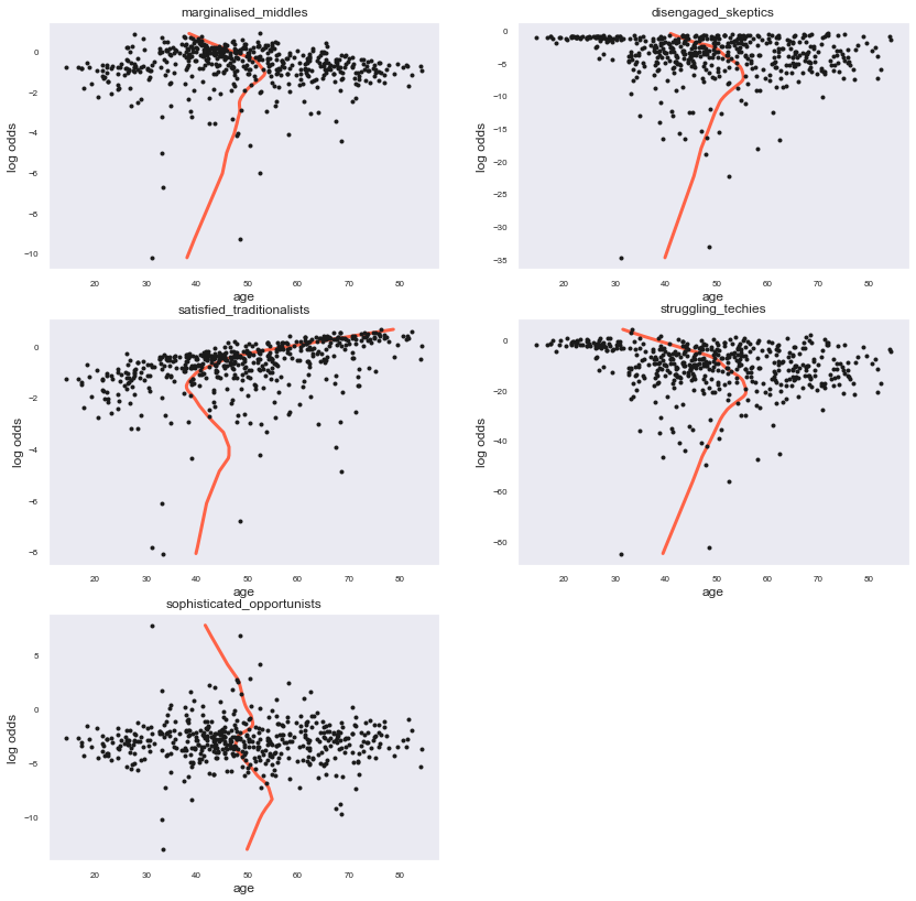
By plotting the independent variable ‘age’ (representing here also the other variables) to the models logodds we can clearly see non-linear relationships for all classes. To document that further we will proceed with a Box Tidwell test and will try transformed versions of this predictor to see if we can achieve an acceptable linearity with a transformed predictor.
# all continuous variables to transform
df_boxtidwell = df_check.copy()
df_boxtidwell = df_boxtidwell.drop(df_boxtidwell[df_boxtidwell.annual_branch_visits == 0].index)
df_boxtidwell = df_boxtidwell.drop(df_boxtidwell[df_boxtidwell.deposit_revenue == 0].index)
df_boxtidwell = df_boxtidwell.drop(df_boxtidwell[df_boxtidwell.annual_income == 0].index)
df_boxtidwell = df_boxtidwell.drop(df_boxtidwell[df_boxtidwell.service_satisfaction_level == 0].index)

# Define continuous variables
z=5
continuous_var = df_boxtidwell.iloc[:, 0:z].columns

# Add logit transform interaction terms (natural log) for continuous variables e.g. Age * Log(Age)
for var in continuous_var:
    df_boxtidwell[f'Transf_{var}'] = df_boxtidwell[var].apply(lambda x: x * np.log(x) ) #np.log = natural log

df_boxtidwell.head()
#continuous_var
cols = continuous_var.append(df_boxtidwell.iloc[:, -z:].columns)
cols
Index(['age', 'annual_income', 'annual_branch_visits',
       'service_satisfaction_level', 'deposit_revenue', 'Transf_age',
       'Transf_annual_income', 'Transf_annual_branch_visits',
       'Transf_service_satisfaction_level',
       'Transf_deposit_revenue'],
      dtype='object')
import statsmodels.api as sm

# Redefine independent variables to include interaction terms
#X_lt = df_boxtidwell[cols[-5:]]
X_lt = df_boxtidwell[cols]
#_lt = df_boxtidwell['deposit_revenue']
y_lt = df_boxtidwell['Segment']

# Add constant
X_lt = sm.add_constant(X_lt, prepend=False)

# Build model and fit the data (using statsmodel's Logit)
logit_result = sm.GLM(y_lt, X_lt, family=sm.families.Binomial()).fit()

# Display summary results
print(logit_result.summary())
                 Generalized Linear Model Regression Results
==============================================================================
Dep. Variable:                Segment   No. Observations:                  488
Model:                            GLM   Df Residuals:                      477
Model Family:                Binomial   Df Model:                           10
Link Function:                  logit   Scale:                          1.0000
Method:                          IRLS   Log-Likelihood:                    nan
Date:                Fri, 10 Dec 2021   Deviance:                       34679.
Time:                        15:42:50   Pearson chi2:                 3.50e+18
No. Iterations:                     7
Covariance Type:            nonrobust
=====================================================================================================
                                        coef    std err          z      P>|z|      [0.025      0.975]
-----------------------------------------------------------------------------------------------------
age                               -8.491e+15   6.72e+06  -1.26e+09      0.000   -8.49e+15   -8.49e+15
annual_income                     -2.671e+13   1.19e+04  -2.24e+09      0.000   -2.67e+13   -2.67e+13
annual_branch_visits              -2.924e+14   3.76e+06  -7.78e+07      0.000   -2.92e+14   -2.92e+14
service_satisfaction_level         3.532e+15   2.36e+07    1.5e+08      0.000    3.53e+15    3.53e+15
deposit_revenue                   -1.562e+14   8.41e+04  -1.86e+09      0.000   -1.56e+14   -1.56e+14
Transf_age                         1.735e+15   1.37e+06   1.27e+09      0.000    1.74e+15    1.74e+15
Transf_annual_income               2.248e+12   1000.974   2.25e+09      0.000    2.25e+12    2.25e+12
Transf_annual_branch_visits        2.267e+14   9.75e+05   2.33e+08      0.000    2.27e+14    2.27e+14
Transf_service_satisfaction_level -1.415e+15   1.13e+07  -1.25e+08      0.000   -1.41e+15   -1.41e+15
Transf_deposit_revenue             2.056e+13   1.01e+04   2.05e+09      0.000    2.06e+13    2.06e+13
const                              2.078e+17   7.07e+07   2.94e+09      0.000    2.08e+17    2.08e+17
=====================================================================================================
The GLM logit_result shows that basically all variables are flagged for non-linearity across all classic transformations by have significant p-values for the regular and tranformed feature variables. This applies also for all other regular transformations. We therefore have to accept that this data is illsuited for such a logistic regression model and rather move on, instead of sinking more time into this.
Overview Logistic Regression assumptions check
| # | Assumption | Check | |—|:—————————————————————————————————————————————————————————————————————————————————————————————————————————————————————————————-:|:—–:| | 1 | Appropriate outcome type - our case will be the multinomial regression where the dependent variable y will have more than two classes of outcomes. | ☑ | | 2 | Logistic regression requires the observations to be independent of each other. In other words, the observations should not come from repeated measurements or matched data. | ☑ | | 3 | Logistic regression requires there to be little or no multicollinearity among the independent variables. This means that the independent variables should not be too highly correlated with each other. | ☑ | | 4 | Logistic regression assumes linearity of independent variables and log odds. although this analysis does not require the dependent and independent variables to be related linearly, it requires that the independent variables are linearly related to the log odds. | ☒ | | 5 | Logistic regression typically requires a large sample size. A general guideline is that you need at minimum of 10 cases with the least frequent outcome for each independent variable in your model. For example, if you have 5 independent variables and the expected probability of your least frequent outcome is .10, then you would need a minimum sample size of 500 (10*5 / .10). | |
Alternative multi-classification with Support Vector Machines extended by cost sensitiveness
So alternatively to Logistic Regression we could pick the popular random forest algorithm, but for a change we go for a classic support vector machine (SVM) model. SVM does not require any assumptions to be met, that is very soothing at this point ;)
Instead of the algorithm selection and model tuning we want to shift focus towards how to integrate costs of misclassification into the model building process, especially with assymmetric multi-missclassfication costs, where some misclassifications are more costly than others. This is where we actually have an optimization problem and a lever to achieve cost savings, which will more or less contribute to the overall segmentation goal of increasing efficieny and effectiveness at the same time.
Different costs for different types of errors
The overall objective in classification is to minimize classification errors, with cost-sensitive classification however this objective is shifted from minimizing classification errors, to rather minimizing type I and type II mis-classification errors where each of the multiple classes are associated with their own cost.
We define a error-cost matrix, in which the entries at each cell $({row}{a}, {column}{b})$ specify how costly it should be to predict class $a$ when the true class is $b$.
import pandas as pd, numpy as np

# assymmetric nonreciprocal costs of classification errors
# true class vs. wrong predicted class costs

true_vs_predicted_class_cost = pd.DataFrame(index=segment_names, columns=segment_names)

true_vs_predicted_class_cost.marginalised_middles       = [0,10,10,10,10]
true_vs_predicted_class_cost.disengaged_skeptics        = [10,0, 10, 10, 10]
true_vs_predicted_class_cost.satisfied_traditionalists  = [10,10, 0, 10, 10]
true_vs_predicted_class_cost.struggling_techies         = [10,10, 10, 0, 10]
true_vs_predicted_class_cost.sophisticated_opportunists = [200,34, 40, 25, 0]

true_vs_predicted_class_cost = true_vs_predicted_class_cost.T # transpose the column-wise-built DataFrames
true_vs_predicted_class_cost
| marginalised_middles | disengaged_skeptics | satisfied_traditionalists | struggling_techies | sophisticated_opportunists | |
|---|---|---|---|---|---|
| marginalised_middles | 0 | 10 | 10 | 10 | 10 |
| disengaged_skeptics | 10 | 0 | 10 | 10 | 10 |
| satisfied_traditionalists | 10 | 10 | 0 | 10 | 10 |
| struggling_techies | 10 | 10 | 10 | 0 | 10 |
| sophisticated_opportunists | 200 | 34 | 40 | 25 | 0 |
# for computation we map the class labels to numeric classes

# map class labels numerically
d = dict([(y,x) for x,y in enumerate((segment_names))])

# convert to numeric indices
true_vs_predicted_class_cost.columns = d.values()
true_vs_predicted_class_cost.index = d.values()

true_vs_predicted_class_cost

import random
true_vs_predicted_class_cost
| 0 | 1 | 2 | 3 | 4 | |
|---|---|---|---|---|---|
| 0 | 0 | 10 | 10 | 10 | 10 |
| 1 | 10 | 0 | 10 | 10 | 10 |
| 2 | 10 | 10 | 0 | 10 | 10 |
| 3 | 10 | 10 | 10 | 0 | 10 |
| 4 | 200 | 34 | 40 | 25 | 0 |
# map observations class string labels to number

# convert to np array
cost_matrix = true_vs_predicted_class_cost.values

try:
    y = [d[s] for s in y]
except:
    print('already done')

# new cost array for package 'costsensitive'
C = np.array([cost_matrix[i] for i in y])
np.random.seed(1)
#C = (np.random.random_sample((500, 5))/100 + 1) * C

#C = np.linalg.inv(C)

# save cost matrix to csv file
# np.savetxt('costmatrix.csv', C, delimiter=',')

C
already done


array([[  0,  10,  10,  10,  10],
       [  0,  10,  10,  10,  10],
       [  0,  10,  10,  10,  10],
       ...,
       [200,  34,  40,  25,   0],
       [200,  34,  40,  25,   0],
       [200,  34,  40,  25,   0]], dtype=int64)
We use a Machine Learning model based on Support Vector Machines to classify the five customer segments based on the clients predictors with the goal to generalize well for new real clients.
In a first step we do a conventional SVM for this imbalanced dataset, for which we use an appropiate metric for evaluation: the weighted F1-Score.
After that we will model the different costs of actual misclassifications of clients into a incorrect segments. This is important because not every error that is made is equally costly. The metric to be evaluated then will be cost savings to the baseline cost of the conventional LR model of Step 1.
Baseline SVM model
from sklearn.model_selection import train_test_split
from sklearn.preprocessing import StandardScaler, MinMaxScaler

#segm = segm.values
X = segm.iloc[:, :segm.shape[1] - 1].astype('float64')
y = segm.iloc[:, segm.shape[1] - 1]

"""# numerical labels
try:
    y = [d[s] for s in y]
except:
    print('already done') """

# numerical labels
nummap = dict(zip(segment_names,range(0,5)))
y = y.map(nummap)
X_train, X_test, C_train, C_test, y_train, y_test = train_test_split(X, C, y, test_size=.5, random_state=0,
                                                                     stratify=y
                                                                    )
scaler = StandardScaler()
scaler.fit(X_train)
X_train = scaler.transform(X_train)
X_test = scaler.transform(X_test)
[[-0.06506306 -1.03252879 -0.535742   -0.52489066 -0.89210993  0.67795498
   0.51868635  0.88640526 -0.0872679 ]
 [-0.73825472  0.968496   -0.75466817 -0.52489066 -0.72250728 -1.89005632
   0.51868635  0.88640526 -0.22493628]]
[[ 0 10 10 10 10]
 [ 0 10 10 10 10]]
71    0
26    0
Name: Segment, dtype: int64
[[ 2.27122869 -1.03252879  0.27819165 -0.52489066  1.56712848  0.67795498
   0.51868635 -1.12815215  0.68012859]
 [-0.94041437 -1.03252879  1.54138938  1.90515869 -0.46810331  0.67795498
   0.51868635 -1.12815215  2.54650874]]
<class 'pandas.core.series.Series'>
(250, 9)
(250, 5)
(250,)
Fitting the classifiers and tracking test set results:
from sklearn import svm
from sklearn.metrics import confusion_matrix

### Keeping track of the results for later
name_algorithm = list()
f1_scores = list()
costs = list()
collect_conf_mat = list()

#### Baseline : Classic SVM with no weights

svm_model = svm.SVC(random_state=1)
svm_model.fit(X_train, y_train)

preds_svm = svm_model.predict(X_test)
from sklearn.metrics import precision_recall_fscore_support, f1_score

conf_mat = confusion_matrix(y_test, preds_svm)

f1 = f1_score(y_test, preds_svm, zero_division=1, average='weighted')
f1
0.9668887073655656
# logging results
name_algorithm.append("Classic Support Vector Machine SVC Method")
f1_scores.append(f1)
# ex post calculation of costs with the baseline model

costs.append( C_test[np.arange(C_test.shape[0]), preds_svm].sum() )
collect_conf_mat.append(confusion_matrix(y_test, preds_svm))
from sklearn.metrics import plot_confusion_matrix

disp = plot_confusion_matrix(svm_model, X_test, y_test,
                                 display_labels=segment_names,
                                 cmap=plt.cm.Blues)
disp.ax_.set_xticklabels(segment_names, size=12, rotation=30, ha='right')
plt.grid(False)
plt.show()
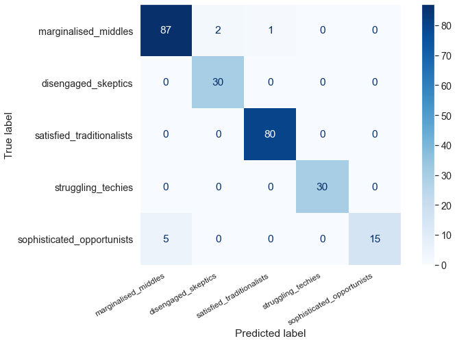
pd.DataFrame(precision_recall_fscore_support(y_test, preds_svm), columns=segment_names, index=['precision', 'recall', 'fscore', 'support'])
| marginalised_middles | disengaged_skeptics | satisfied_traditionalists | struggling_techies | sophisticated_opportunists | |
|---|---|---|---|---|---|
| precision | 0.945652 | 0.937500 | 0.987654 | 1.0 | 1.000000 |
| recall | 0.966667 | 1.000000 | 1.000000 | 1.0 | 0.750000 |
| fscore | 0.956044 | 0.967742 | 0.993789 | 1.0 | 0.857143 |
| support | 90.000000 | 30.000000 | 80.000000 | 30.0 | 20.000000 |
Fitting cost-sensitive classifiers
The algorithms applied here are reduction methods that turn our classification-cost problem into a series of importance-weighted binary classification sub-problems (‘multi oracle call’), see for the details the documentation https://costsensitive.readthedocs.io/en/latest/
Github: https://github.com/david-cortes/costsensitive/
One theoretical algorithm implemented in that package originates here: Beygelzimer, A., Dani, V., Hayes, T., Langford, J., & Zadrozny, B. (2005, August). Error limiting reductions between classification tasks. http://citeseerx.ist.psu.edu/viewdoc/download?doi=10.1.1.90.2161&rep=rep1&type=pdf
from costsensitive import WeightedAllPairs, WeightedOneVsRest, RegressionOneVsRest, FilterTree, CostProportionateClassifier
from sklearn import svm

### 1: WAP = Weighted All-Pairs as described in "Error limiting reductions between classification tasks"

costsensitive_WAP = WeightedAllPairs(svm.SVC(random_state=1), weigh_by_cost_diff=False)
costsensitive_WAP.fit(X_train, C_train)
preds_WAP = costsensitive_WAP.predict(X_test, method = 'most-wins')
f1_WAP = f1_score(y_test, preds_WAP, zero_division=1, average='weighted')
# log
collect_conf_mat.append(confusion_matrix(y_test, preds_WAP))
name_algorithm.append("Weighted All-Pairs SVM 'Error limiting reductions between classification tasks'")
f1_scores.append(f1_WAP)
costs.append(C_test[np.arange(C_test.shape[0]), preds_WAP].sum())


#### 2: WAP2 = Weighted All-Pairs - cost difference weights enabled

costsensitive_WAP2 = WeightedAllPairs(svm.SVC(random_state=1), weigh_by_cost_diff=True)
costsensitive_WAP2.fit(X_train, C_train)
preds_WAP2 = costsensitive_WAP2.predict(X_test)
f1_WAP2 = f1_score(y_test, preds_WAP2, zero_division=1, average='weighted')
# log
collect_conf_mat.append(confusion_matrix(y_test, preds_WAP2))
name_algorithm.append("Weighted All-Pairs SVM - cost difference weights enabled")
f1_scores.append(f1_WAP2)
costs.append( C_test[np.arange(C_test.shape[0]), preds_WAP2].sum() )


#### 3: WOR = Weighted One-Vs-Rest heuristic with simple cost-weighting schema

costsensitive_WOR = WeightedOneVsRest(svm.SVC(random_state=1), weight_simple_diff=True)
costsensitive_WOR.fit(X_train, C_train)
preds_WOR = costsensitive_WOR.predict(X_test)
f1_WOR = f1_score(y_test, preds_WOR, zero_division=1, average='weighted')
# log
collect_conf_mat.append(confusion_matrix(y_test, preds_WOR))
name_algorithm.append("Weighted One-Vs-Rest SVM, simple cost-weighting schema")
f1_scores.append(f1_WOR)
costs.append( C_test[np.arange(C_test.shape[0]), preds_WOR].sum() )
Optimization Results Comparison
numplots = len(collect_conf_mat)
#print(numplots)
fig, ax = plt.subplots(numplots,1, sharey=True, figsize=(4,17))
#ax[0].get_shared_x_axes().join(ax[1])
for c in range(0,numplots):
    #ax[0].get_shared_x_axes().join(ax[c])
    sns.heatmap(collect_conf_mat[c], yticklabels=segment_names, annot=True, ax=ax[c], cmap=plt.cm.Blues, cbar=False)
    ax[c].set_title(name_algorithm[c],loc='center', fontsize=13)
    #plt.title(drop_combos[c], loc='center', fontsize=5)
    ax[numplots-1].set_xlabel("Predicted")
    ax[c].set_ylabel("True")
    ax[numplots-1].set_xticklabels(segment_names, fontsize=12, rotation=35, ha='right')

#fig.tight_layout(h_pad=2)
plt.subplots_adjust(hspace=0.3)
fig.suptitle('Confusion Matrix Comparison', fontsize = 22)
plt.subplots_adjust(top=0.9)
plt.show()
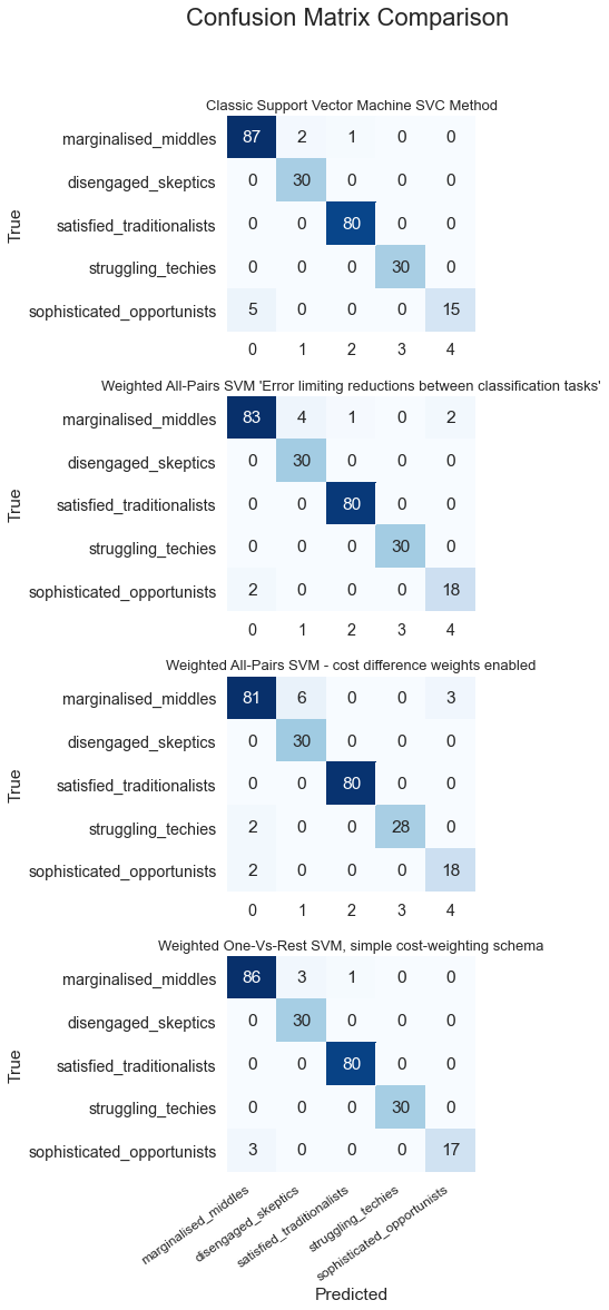
import pandas as pd

results = pd.DataFrame({
    'Method' : name_algorithm,
    'F1' : f1_scores,
    'Total_Cost' : costs
})
results=results[['Method', 'Total_Cost', 'F1']]
results.set_index('Method')
| Total_Cost | F1 | |
|---|---|---|
| Method | ||
| Classic Support Vector Machine SVC Method | 1030 | 0.966889 |
| Weighted All-Pairs SVM 'Error limiting reductions between classification tasks' | 470 | 0.963998 |
| Weighted All-Pairs SVM - cost difference weights enabled | 510 | 0.948454 |
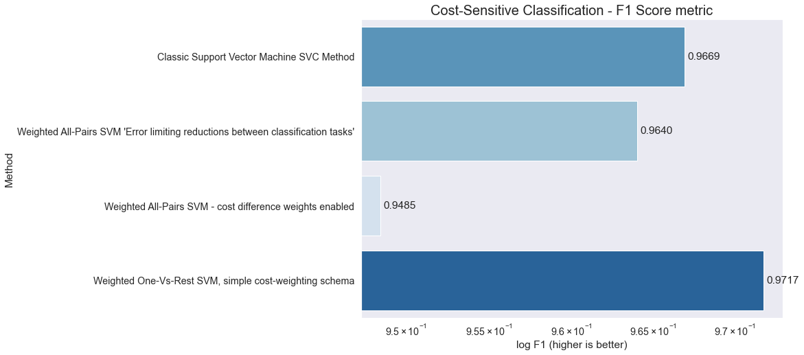
| Weighted One-Vs-Rest SVM, simple cost-weighting schema | 640 | 0.971733 |
import matplotlib.pyplot as plt
import seaborn as sns
#%matplotlib inline

rank = results.F1.sort_values().index
palette = sns.color_palette('Blues', len(rank))


fig = plt.gcf()
fig.set_size_inches(11, 8)
sns.set(font_scale=1.3)
ax = sns.barplot(x = "F1", y = "Method", data = results, palette=np.array(palette)[rank])
ax.set(xlabel='log F1 (higher is better)')
# data bar annotations
for p in ax.patches:
    ax.annotate("%.4f" % p.get_width(), xy=(p.get_width(), p.get_y()+p.get_height()/2),
            xytext=(5, 0), textcoords='offset points', ha="left", va="center")

ax.set_xscale("log")
plt.title('Cost-Sensitive Classification - F1 Score metric', fontsize=20)
plt.show()
import matplotlib.pyplot as plt
import seaborn as sns
sns.set_style('dark')
#%matplotlib inline

rank = results['Total_Cost'].sort_values(ascending=False).index
palette = sns.color_palette('Blues', len(rank))

fig = plt.gcf()
fig.set_size_inches(11, 8)
sns.set(font_scale=1.3)
ax = sns.barplot(x = "Total_Cost", y = "Method", data = results, palette=np.array(palette)[rank])
ax.set(xlabel='Total Cost (lower is better)')
# data bar annotations
for p in ax.patches:
    ax.annotate("%.0f" % p.get_width(), xy=(p.get_width(), p.get_y()+p.get_height()/2),
            xytext=(5, 0), textcoords='offset points', ha="left", va="center")

plt.title('Cost-Sensitive Classification - Total Cost metric', fontsize=20)
plt.show()
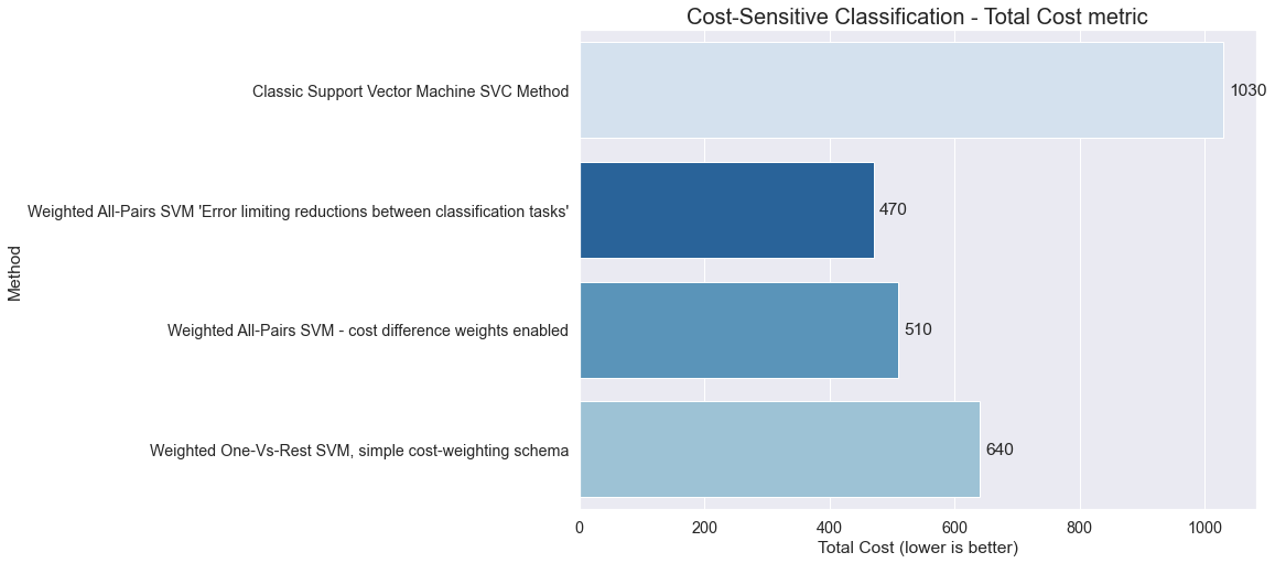
results
| Method | Total_Cost | F1 | |
|---|---|---|---|
| 0 | Classic Support Vector Machine SVC Method | 1030 | 0.966889 |
| 1 | Weighted All-Pairs SVM 'Error limiting reducti... | 470 | 0.963998 |
| 2 | Weighted All-Pairs SVM - cost difference weigh... | 510 | 0.948454 |
| 3 | Weighted One-Vs-Rest SVM, simple cost-weightin... | 640 | 0.971733 |
results = results.assign(CostSavings = lambda x: (x['Total_Cost'] - results.loc[0,'Total_Cost']) * -1)
results = results.assign(F1_Deviation = lambda x: (x['F1'] - results.loc[0,'F1']))
results
| Method | Total_Cost | F1 | CostSavings | F1_Deviation | |
|---|---|---|---|---|---|
| 0 | Classic Support Vector Machine SVC Method | 1030 | 0.966889 | 0 | 0.000000 |
| 1 | Weighted All-Pairs SVM 'Error limiting reducti... | 470 | 0.963998 | 560 | -0.002891 |
| 2 | Weighted All-Pairs SVM - cost difference weigh... | 510 | 0.948454 | 520 | -0.018435 |
| 3 | Weighted One-Vs-Rest SVM, simple cost-weightin... | 640 | 0.971733 | 390 | 0.004845 |
import matplotlib.pyplot as plt
import seaborn as sns
sns.set_style('dark')
#%matplotlib inline

rank = results.iloc[1:,:]['CostSavings'].sort_values(ascending=True).index
rank2 = results.iloc[1:,:]['F1_Deviation'].sort_values(ascending=True).index
palette = sns.color_palette('Blues', len(rank))
palette2 = sns.color_palette('Reds', len(rank))

fig = plt.gcf()
fig.set_size_inches(11, 8)
sns.set(font_scale=1.3)
ax = sns.barplot(x = "CostSavings", y = "Method", data = results.iloc[1:,:], palette=np.array(palette)[rank-1])

ax.set(xlabel='Cost Savings (higher is better)')
ax2 = ax.twiny()
def change_width(ax, new_value) :
    locs = ax.get_yticks()
    for i,patch in enumerate(ax.patches):
        current_width = patch.get_width()
        diff = current_width - new_value
        # we change the bar width
        patch.set_height(new_value)
        # we recenter the bar
        patch.set_y(locs[i] - (new_value * .5))


ax2 = sns.barplot(x = "F1_Deviation", y = "Method", data = results.iloc[1:,:], palette=np.array(palette2)[rank2-1], ax=ax2)
ax2.set(xlabel='F1_Deviation (higher is better)')
change_width(ax2, .25)

plt.title('Comparison of Cost Sensitive Methods to the Baseline Model\n', fontsize=20)
plt.legend(['F1 Score Deviation', 'Cost Saving'], labelcolor=['crimson','royalblue'], loc='lower left', edgecolor='white')
plt.axvline(0, 0, color='crimson')
plt.show()
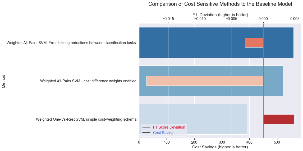
We can summarize that cost savings can be significant out of the box and may be possible even with a higher F1 Score. With further tuning efforts this may become however much more like a trade-off decision. And the question how far you want to favor marginal cost savings over lower F1-Score or Accuracy results.