Non Fungible Token (NFT) Rarity Analysis with Jaccard Distance
trait set distance calculation with Jaccard Similarity/Distance
Overview market macro stats for a market & collection of my choice
# api market macro stats
# for collection officialtimelessapeclub
# on opensea market
import requests, json

url_stats = "https://api.opensea.io/api/v1/collection/officialtimelessapeclub/stats"

r = requests.get(url_stats)

print(f"floor price:", r.json()["stats"]["floor_price"],f"ETH")
print(f"24h Volume:", r.json()["stats"]["one_day_volume"],f"ETH")
print(f"24h sales:", r.json()["stats"]["one_day_sales"])

print(f"Number of sales in last 30 days", r.json()["stats"]["thirty_day_sales"])
print(f"24h AVG price:", r.json()["stats"]["one_day_average_price"],f"ETH")
print(f"Unique owners:", r.json()["stats"]["num_owners"],f"/", r.json()["stats"]["count"] )
floor price: 0.04 ETH
24h Volume: 0.6194999999999999 ETH
24h sales: 15.0
Number of sales in last 30 days 1426.0
24h AVG price: 0.041299999999999996 ETH
Unique owners: 2168 / 4645.0
import pandas as pd
asset_traits = pd.read_pickle('asset_traits.pkl') # load prepared df with trait variants of tokens 0 to 4094
asset_traits.head()
| token_id | MOUTH | HAT | EYES | CLOTH | BACKGROUND | SKIN | WATCH | LEGENDARY APE | |
|---|---|---|---|---|---|---|---|---|---|
| 0 | 0 | Bubblegum | Trucker | 3D | Astronaut | Cream | Brown | Bartier Cantos | NaN |
| 1 | 1 | Smirk | Beanie | Frown | Bulletproof Vest | Cream | Gray | Robin Sub | NaN |
| 2 | 2 | Bubblegum | Jungle | Star | Army | Light Green | Gray | Parrot Lumos | NaN |
| 3 | 3 | Disappointed | Bunny | Sad | Tshirt | Light Green | Blue | Cartoon | NaN |
| 4 | 4 | Disappointed | Boat | Bored | Singlet | Sea Green | Gold | Berry Rose | NaN |
Now we want to compare each token id and its specific trait set to all other tokens and see how different each token really is compared to all other tokens. We apply here the concept of Jaccard Similarity and Distance which are defined as follows:
\[Jaccard Similarity: J = \frac{|A \cap B|}{|A \cup B|} = \frac{|A \cap B|}{|A| + |B| – |A \cup B|}\] \[Jaccard Distance: d_J = \frac{|A \cup B| – |A \cap B|}{|A \cup B|} = 1 – J(A, B)\]We use the Jaccard Distance to measures dissimilarity between its traits and every other token trait set in the same collection. The Jaccard distance facilitates the symmetric difference of the two sets and measures its size, which is put into relation to the union (of these two sets).
I have optimized these numerous iterations of rows with df.itertuples() already, but still thinking on how to implement the same completely vectorized, if that is possible.
Update 1 - 03-Mar-22:
- Label encoding trait variants
- Implementing Multiprocessing Pool (spawn processes for DataFrame chunks)
# Update 1 - 03-Mar-22
# map trait variants to short number codes before number crunching to save 40%+ processing time

dftest = asset_traits.copy()

# all unique trait variants
u =set()
for col in dftest.iloc[:,1:].columns:
    dftest[col] = dftest[col].fillna(0)
    v = set(dftest[col].unique())
    u = u.union(v)

# map unique code across all cols to all trait variants
mapping = {item:i for i, item in enumerate(u)}

for col in dftest.iloc[:,1:].columns:
    dftest[col] = dftest[col].apply(lambda x: mapping[x])

dftest.head()
| token_id | MOUTH | HAT | EYES | CLOTH | BACKGROUND | SKIN | WATCH | LEGENDARY APE | |
|---|---|---|---|---|---|---|---|---|---|
| 0 | 0 | 75 | 120 | 96 | 34 | 22 | 118 | 62 | 0 |
| 1 | 1 | 91 | 63 | 19 | 109 | 22 | 78 | 101 | 0 |
| 2 | 2 | 75 | 84 | 64 | 3 | 114 | 78 | 90 | 0 |
| 3 | 3 | 89 | 42 | 33 | 102 | 114 | 106 | 13 | 0 |
| 4 | 4 | 89 | 44 | 80 | 11 | 73 | 2 | 88 | 0 |
%%time
# Update 1 - 03-Mar-22
# multiprocessing pool for the cpu intensive jaccard distances calculations

import multiprocessing
#from multiprocessing import Pool
from itertools import repeat
import pandas as pd
import jaccard # moved jaccard distance calculations code as jaccard function to jaccard.py in order to make multiproc work

collection_slug = 'officialtimelessapeclub'

# Divide asset dataframe into n chunks
n = 6 # define the number of processes (cpu cores)
chunk_size = int(asset_traits.shape[0]/n)+1
chunks = [asset_traits.index[i:i + chunk_size] for i in range(0, asset_traits.shape[0], chunk_size)]

# multiprocess pool - sending chunk indices and collection info as args, df opened directly by jaccard.py
with multiprocessing.Pool() as pool:
    result = pool.starmap(jaccard.jaccard, zip(chunks, repeat(collection_slug)))

# Concatenate all chunks back to one
jdist = pd.concat(result)
Wall time: 2min 11s
Saving approx. 75% time compared to the single thread code.
%%time
# original single thread solution

import numpy as np
from scipy.spatial.distance import jaccard
import warnings
warnings.simplefilter(action='ignore', category=FutureWarning)
# https://stackoverflow.com/questions/40659212/futurewarning-elementwise-comparison-failed-returning-scalar-but-in-the-futur

df2 = asset_traits.copy()

jdist = pd.DataFrame(columns=['token_id','jd_mean'])

# calc jaccard dist for each row
for row1 in df2.itertuples():
    jdlist = []
    # calc against all other rows
    for row2 in df2.itertuples():
        if row1.token_id != row2.token_id:
            jd = jaccard( np.array(row1[2:]), np.array(row2[2:]) ) # jaccard distance
            jdlist.append(jd)
    jdist.loc[row1.token_id] = [row1.token_id, np.mean(jdlist)] # save the mean of jd of row1
Wall time: 9min 40s
# normalize jaccard distances for a score 0 to 1
from sklearn import preprocessing
from sklearn.preprocessing import MinMaxScaler

scaler = MinMaxScaler()
arr = jdist['jd_mean'].to_numpy()
normalized = scaler.fit_transform(arr.reshape(-1, 1))
# write to df
score = pd.DataFrame(columns=['token_id','score'])
score['token_id'] = jdist['token_id']
score['score'] = normalized
from scipy import stats
zscores = stats.zscore(arr)
import matplotlib.pyplot as plt
import seaborn as sns
sns.set_style('darkgrid')

plt.figure(figsize=(15,4))
sns.histplot(data=score.score)
plt.title('Normalized scores 0 to 1')
plt.show()
plt.figure(figsize=(15,4))
sns.histplot(data=zscores)
plt.title('z-scores of Jaccard distance means')
plt.show()
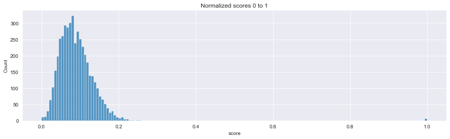
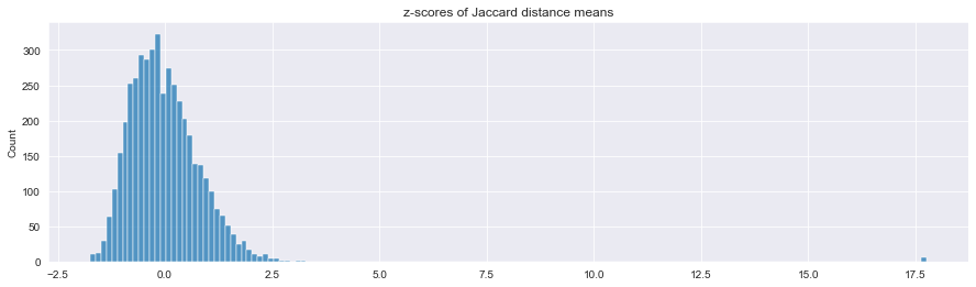
It becomes obvious of how skewed the distribution of tokens is and how dissimilar the legendary apes on the right really are in this collection, that is 17 standard deviations!
# normalized scores as score
# and the arithmetic mean of the original jaccard dissimilarities (distances)
score['jdist_mean'] = jdist.jd_mean
score.head()
| token_id | score | jdist_mean | |
|---|---|---|---|
| 0 | 0 | 0.085865 | 6.452084 |
| 1 | 1 | 0.040798 | 6.376137 |
| 2 | 2 | 0.104821 | 6.484028 |
| 3 | 3 | 0.068918 | 6.423524 |
| 4 | 4 | 0.117876 | 6.506029 |
score.to_pickle('score.pkl') # save score df to file
# best score 1
score.sort_values('score', ascending=False)
| token_id | score | jdist_mean | |
|---|---|---|---|
| 3623 | 3623.0 | 1.000000 | 7.992449 |
| 2533 | 2533.0 | 1.000000 | 7.992449 |
| 106 | 106.0 | 1.000000 | 7.992449 |
| 3888 | 3888.0 | 1.000000 | 7.992449 |
| 1836 | 1836.0 | 1.000000 | 7.992449 |
| ... | ... | ... | ... |
| 916 | 916 | 0.004328 | 6.317152 |
| 332 | 332 | 0.003526 | 6.315804 |
| 3251 | 3251 | 0.002565 | 6.314186 |
| 3068 | 3068 | 0.000641 | 6.310949 |
| 1510 | 1510 | 0.000000 | 6.309871 |
3709 rows × 3 columns
# let's rank the scores with pandas rank
score['rank'] = score['score'].rank(method='min', ascending=False)
score.sort_values('rank', ascending=True)
| token_id | score | jdist_mean | rank | |
|---|---|---|---|---|
| 106 | 106.0 | 1.000000 | 7.992449 | 1.0 |
| 1836 | 1836.0 | 1.000000 | 7.992449 | 1.0 |
| 3623 | 3623.0 | 1.000000 | 7.992449 | 1.0 |
| 2533 | 2533.0 | 1.000000 | 7.992449 | 1.0 |
| 3888 | 3888.0 | 1.000000 | 7.992449 | 1.0 |
| ... | ... | ... | ... | ... |
| 916 | 916 | 0.004328 | 6.317152 | 3705.0 |
| 332 | 332 | 0.003526 | 6.315804 | 3706.0 |
| 3251 | 3251 | 0.002565 | 6.314186 | 3707.0 |
| 3068 | 3068 | 0.000641 | 6.310949 | 3708.0 |
| 1510 | 1510 | 0.000000 | 6.309871 | 3709.0 |
3709 rows × 4 columns
#let's check a specific token for its rank
score.loc[['1081']]
# token 1081 is pretty average:
| token_id | score | jdist_mean | rank | |
|---|---|---|---|---|
| 1081 | 1081 | 0.076294 | 6.438242 | 2100.0 |
# let us check the current market what rarities are offered at which prices
# for that we have to scrape due to lack of immeadiately available api key
# which is required for the 'Retrieving assets' api call
# https://docs.opensea.io/reference/getting-assets

import requests
import cloudscraper # can scrape cloudflare sites

scraper = cloudscraper.create_scraper(
    browser={
        'browser': 'firefox',
        'platform': 'windows',
        'mobile': False
    }
)
from bs4 import BeautifulSoup as bs
url = "https://opensea.io/collection/officialtimelessapeclub?search[sortAscending]=true&search[sortBy]=PRICE&search[toggles][0]=BUY_NOW"
r = scraper.get(url).text
# todo: change to selenium to better deal with opensea uses infinity scrolling

import re
market = pd.DataFrame(columns=['token_id', 'price', 'rank', 'price_rank_product'])

html_code = bs(r, 'html.parser')
cards = html_code.find_all('article', class_=re.compile('^AssetSearchList--asset'))

for c in cards:
    price = c.find('div', class_=re.compile('^Price--amount')).getText(strip=True).split("#",1)[0] if c.find('div', class_=re.compile('^Price--amount')) else "none"
    token = c.find('div', class_=re.compile('^AssetCardFooter--name')).getText(strip=True).split("#",1)[1] if c.find('div', class_=re.compile('^AssetCardFooter--name')) else "none"

    token_score = tmp.loc[tmp.token_id == token]['rank'].to_numpy()

    # todo: change to selenium to better deal with opensea uses infinity scrolling
    if len(token_score) == 1:
        grade = round(float(price) * token_score[0],1)
    else: #lazy loaded cards
        token_score = str(token_score)
        grade = '-----'
    market.loc[len(market.index)] = [token, price, token_score, grade]
market[0:32].sort_values('price')
| token_id | price | rank | price_rank_product | |
|---|---|---|---|---|
| 0 | 1328 | 0.05 | [3064] | 153.2 |
| 1 | 3073 | 0.05 | [3064] | 153.2 |
| 2 | 1220 | 0.05 | [1331] | 66.6 |
| 3 | 209 | 0.05 | [3440] | 172.0 |
| 4 | 210 | 0.055 | [3496] | 192.3 |
| 5 | 208 | 0.059 | [1576] | 93.0 |
| 6 | 1092 | 0.059 | [2908] | 171.6 |
| 8 | 3348 | 0.06 | [1745] | 104.7 |
| 7 | 3290 | 0.06 | [2830] | 169.8 |
| 9 | 212 | 0.064 | [2117] | 135.5 |
| 10 | 3685 | 0.065 | [2813] | 182.8 |
| 11 | 1091 | 0.069 | [1864] | 128.6 |
| 12 | 966 | 0.069 | [1454] | 100.3 |
| 13 | 1869 | 0.069 | [1138] | 78.5 |
| 19 | 1240 | 0.07 | [2873] | 201.1 |
| 20 | 1430 | 0.07 | [3306] | 231.4 |
| 18 | 780 | 0.07 | [2379] | 166.5 |
| 15 | 534 | 0.07 | [1507] | 105.5 |
| 16 | 3044 | 0.07 | [2547] | 178.3 |
| 14 | 257 | 0.07 | [2971] | 208.0 |
| 17 | 3995 | 0.07 | [3647] | 255.3 |
| 21 | 1080 | 0.075 | [2288] | 171.6 |
| 22 | 1081 | 0.075 | [2100] | 157.5 |
| 23 | 2811 | 0.075 | [2254] | 169.0 |
| 24 | 677 | 0.075 | [2262] | 169.6 |
| 30 | 2833 | 0.08 | [1996] | 159.7 |
| 25 | 166 | 0.08 | [1758] | 140.6 |
| 26 | 770 | 0.08 | [2112] | 169.0 |
| 27 | 1116 | 0.08 | [2918] | 233.4 |
| 28 | 1455 | 0.08 | [824] | 65.9 |
| 29 | 49 | 0.08 | [1618] | 129.4 |
| 31 | 1017 | 0.08 | [3393] | 271.4 |
# voila, pick the best deals
market[0:32].sort_values('price_rank_product').head()
# metric still need calibration and weighting as required
| token_id | price | rank | price_rank_product | |
|---|---|---|---|---|
| 28 | 1455 | 0.08 | [824] | 65.9 |
| 2 | 1220 | 0.05 | [1331] | 66.6 |
| 13 | 1869 | 0.069 | [1138] | 78.5 |
| 5 | 208 | 0.059 | [1576] | 93.0 |
| 12 | 966 | 0.069 | [1454] | 100.3 |