Supply Chain Inventory Reorder Policy Comparison - Monte Carlo Simulation, Bayesian Optimization & Tuning

18 December 2022 - 22 mins read time
Tags: Supply Chain Inventory management Monte Carlo Simulation Bayesian Optimization 3D Visualization Parallelized Processing Python

Having worked with interesting product demand data and the implementation of the product’s reorder policies and related costs, I felt driven to update and improve the Jupyter notebook of the author Mehul. He featured this notebook on his tds article: Inventory Management — Dealing with unpredictable demand. Although the notebook seemed unfinished I addressed a few important pieces: Multiprocessing Performance improvement, Improved Visualization and the required Bayesian Optimization update to version 1.3.

1. Performance improvement through multi processing

The notebook uses a this original function to calculate a large number of combinations of the reorder policy variables q representing the order quantity and r for the reorder point, when orders are to be placed. Unfortunately this was implemented as nested for loops, with the consequence that just one thread is used to calculate the whole grid.

Therefore I came up with this multiprocessing implementation below using the multiprocessing methods pools and starmap to have multiple instances invoked each starting the calculation with a subset chunk of designated variable space to be computed in parallel. For that the function has to be split up into the main invoking function and a subprocess function.

The calculation with a step-size 10 grid took over 30 mins with the original single thread code.

With multiprocessing and n=4 vcores available and specified the calculation took on datacamp workspace 8.5 mins and nearly 10 mins on azure ml with a compute resource standard-F4s-v2.

Doing this later on a local compute with n=10 threads, I hope to achieve significantly below half that. So why not use all the extra cores available? Just do it!

2. Bayesian optimization package comparison

Having not come across the GPyOpt package yet, i was curious how it does compare to the familiar bayes_opt package in terms of optimization, results and handling.

For some unknown reason the function was targeted to be minimized with the GPyOpt package, that is something I was going to change right away. The bounds of the variable space can be set as a ‘discrete type’ variable, that is quite a positive feature as we assume all parameters are indivisable and not continous. By nature of bayesian optimization, gaussian processes do work with continuous number scales and therefore this needs to be addressed by the package itself or by ourselves using them. So unlike GPyOpt in bayes_opt there needs to be provisions to make parameters discrete.

Original implementation with GPyOpt package

product = Product(4)
def fn(args):
    M = args[0][0]
    
    p_list, o_list = mc_simulation(product, M, 500)
    
    print(f' M : {M}, Profit : ${np.mean(p_list):.2f}') 
    return -np.mean(p_list)

from GPyOpt.methods import BayesianOptimization

bounds = [{'name':'M', 'type':'discrete', 'domain': range(10,10000)}]

Op = BayesianOptimization(f = fn,
                         domain = bounds,
                         model_type = 'GP',
                         acquisition_type = 'EI',
                         exact_feval = False,
                         maximize = False,
                         normalize_Y = False)

Op.run_optimization(max_iter=100)

 M : 8564.0, Profit : $-62147.29
 M : 4575.0, Profit : $156476.17
 M : 2384.0, Profit : $279090.77
 M : 1240.0, Profit : $319304.16
 M : 2762.0, Profit : $254034.81
 M : 2379, Profit : $278839.29
 M : 2380, Profit : $281127.72
 M : 1297, Profit : $321277.65
 M : 1303, Profit : $322316.54
 M : 1309, Profit : $318693.07
 M : 1305, Profit : $323975.37
 M : 1311, Profit : $319215.17
 M : 1307, Profit : $320363.83
 M : 1307, Profit : $318037.02

Op.x_opt

array([1305.])

So best parameter is M = 1305 with a simulated Profit of rounded 324K.

So this is straight forward and not many iterations of optimization needed, of course there was only a single parameter.

Let’s check out bayes_opt: we introduce the discretizer function that converts any parameter to integer before it is simulated with. Its result is fed into the optimization function only changed in name. More changes of course in setting up the optimization methods themselves and of course properly setting a fixed random state for the Random Number Generator in numpy.

The periodic review result was not tuned at all; I will invest a little time into reaching the same results in the following continuous review policy optimization thereafter instead.

Comparative implementation with bayes_opt package

!pip show bayesian-optimization 

Name: bayesian-optimization

Version: 1.3.0

Summary: Bayesian Optimization package

Home-page: https://github.com/fmfn/BayesianOptimization

Author: Fernando Nogueira

Author-email: fmfnogueira@gmail.com

License: UNKNOWN

Location: /anaconda/envs/azureml_py38/lib/python3.8/site-packages

Requires: scipy, scikit-learn, numpy

Required-by:

product = Product(4)
def optimization_periodic_review(M):
        
    p_list, o_list = mc_simulation(product, M, 500)
    
    print(f' M : {M}, Profit : ${np.mean(p_list):.2f}') 
    return np.mean(p_list)

def discretizer_periodic_review(M):
    """
    Converts parameters to discrete integers
    """
    M = int(M)
    return optimization_periodic_review(M)

from bayes_opt import BayesianOptimization
import numpy as np
np.random.seed(1)

Op = BayesianOptimization(f = discretizer_periodic_review,
                         pbounds = {'M': (10, 10000)},
                         verbose=2,
                         random_state=1
                         )

Op.maximize(
    acq='poi', 
)

|   iter    |  target   |     M     |
-------------------------------------
 M : 4176, Profit : $183110.60
| [0m1        [0m | [0m1.831e+05[0m | [0m4.176e+03[0m |
 M : 7206, Profit : $12554.08
| [0m2        [0m | [0m1.255e+04[0m | [0m7.206e+03[0m |
 M : 11, Profit : $222172.20
| [95m3        [0m | [95m2.222e+05[0m | [95m11.14    [0m |
 M : 3030, Profit : $244387.35
| [95m4        [0m | [95m2.444e+05[0m | [95m3.03e+03 [0m |
 M : 1476, Profit : $321187.96
| [95m5        [0m | [95m3.212e+05[0m | [95m1.476e+03[0m |
 M : 7505, Profit : $-835.62
| [0m6        [0m | [0m-835.6   [0m | [0m7.505e+03[0m |
 M : 1488, Profit : $319393.86
| [0m7        [0m | [0m3.194e+05[0m | [0m1.489e+03[0m |
 M : 1462, Profit : $319562.57
| [0m8        [0m | [0m3.196e+05[0m | [0m1.462e+03[0m |
 M : 1475, Profit : $319002.68
| [0m9        [0m | [0m3.19e+05 [0m | [0m1.476e+03[0m |
 M : 1485, Profit : $321189.25
| [95m10       [0m | [95m3.212e+05[0m | [95m1.485e+03[0m |
 M : 1476, Profit : $317404.60
| [0m11       [0m | [0m3.174e+05[0m | [0m1.476e+03[0m |
 M : 1488, Profit : $319562.87
| [0m12       [0m | [0m3.196e+05[0m | [0m1.488e+03[0m |
 M : 1268, Profit : $320144.59
| [0m13       [0m | [0m3.201e+05[0m | [0m1.268e+03[0m |
 M : 1485, Profit : $318045.90
| [0m14       [0m | [0m3.18e+05 [0m | [0m1.485e+03[0m |
 M : 9284, Profit : $-98923.86
| [0m15       [0m | [0m-9.892e+0[0m | [0m9.284e+03[0m |
 M : 1484, Profit : $319276.84
| [0m16       [0m | [0m3.193e+05[0m | [0m1.485e+03[0m |
 M : 5819, Profit : $92025.95
| [0m17       [0m | [0m9.203e+04[0m | [0m5.819e+03[0m |
 M : 6890, Profit : $28877.20
| [0m18       [0m | [0m2.888e+04[0m | [0m6.891e+03[0m |
 M : 1475, Profit : $318941.54
| [0m19       [0m | [0m3.189e+05[0m | [0m1.476e+03[0m |
 M : 1485, Profit : $317317.92
| [0m20       [0m | [0m3.173e+05[0m | [0m1.485e+03[0m |
 M : 4500, Profit : $161056.31
| [0m21       [0m | [0m1.611e+05[0m | [0m4.501e+03[0m |
 M : 1488, Profit : $319044.52
| [0m22       [0m | [0m3.19e+05 [0m | [0m1.489e+03[0m |
 M : 9455, Profit : $-110794.55
| [0m23       [0m | [0m-1.108e+0[0m | [0m9.455e+03[0m |
 M : 6280, Profit : $64849.41
| [0m24       [0m | [0m6.485e+04[0m | [0m6.281e+03[0m |
 M : 253, Profit : $254778.76
| [0m25       [0m | [0m2.548e+05[0m | [0m253.9    [0m |
 M : 3090, Profit : $241283.50
| [0m26       [0m | [0m2.413e+05[0m | [0m3.091e+03[0m |
 M : 1476, Profit : $320210.25
| [0m27       [0m | [0m3.202e+05[0m | [0m1.476e+03[0m |
 M : 8495, Profit : $-54828.62
| [0m28       [0m | [0m-5.483e+0[0m | [0m8.496e+03[0m |
 M : 496, Profit : $279645.54
| [0m29       [0m | [0m2.796e+05[0m | [0m496.7    [0m |
 M : 7947, Profit : $-30404.68
| [0m30       [0m | [0m-3.04e+04[0m | [0m7.947e+03[0m |
=====================================

help(Op.maximize)

Help on method maximize in module bayes_opt.bayesian_optimization:

maximize(init_points=5, n_iter=25, acq='ucb', kappa=2.576, kappa_decay=1, kappa_decay_delay=0, xi=0.0, **gp_params) method of bayes_opt.bayesian_optimization.BayesianOptimization instance
    Probes the target space to find the parameters that yield the maximum
    value for the given function.
    
    Parameters
    ----------
    init_points : int, optional(default=5)
        Number of iterations before the explorations starts the exploration
        for the maximum.
    
    n_iter: int, optional(default=25)
        Number of iterations where the method attempts to find the maximum
        value.
    
    acq: {'ucb', 'ei', 'poi'}
        The acquisition method used.
            * 'ucb' stands for the Upper Confidence Bounds method
            * 'ei' is the Expected Improvement method
            * 'poi' is the Probability Of Improvement criterion.
    
    kappa: float, optional(default=2.576)
        Parameter to indicate how closed are the next parameters sampled.
            Higher value = favors spaces that are least explored.
            Lower value = favors spaces where the regression function is
            the highest.
    
    kappa_decay: float, optional(default=1)
        `kappa` is multiplied by this factor every iteration.
    
    kappa_decay_delay: int, optional(default=0)
        Number of iterations that must have passed before applying the
        decay to `kappa`.
    
    xi: float, optional(default=0.0)
        [unused]

Op.max

{'target': 321189.24580837705, 'params': {'M': 1485.1574175844548}}

plt.plot(Op.space.target, label='Op Optimized Profits of Product 4')
plt.title('Iterations of Op bayesian optimization - Periodic Review Policy')
plt.legend()
plt.xlabel('Iteration')
plt.ylabel('Profit')
plt.show()

png

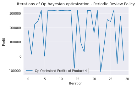
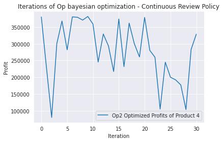
Below the same in green just for the more interesting Continuous Review policy. With a certain amount of tuning I was able to top the previous result with a caveat: the solution consisted in float numbers instead integers. As soon as rounding to the nearest integer, the solution was not better anymore. Haha!

While this would not probably matter for this kind of product, you could imagine a high value product where only a few units are stocked (e.g. below 10). Rounding up or down could have a much higher impact than just a few hundred bucks bottom line.

Continuous Review

def discretizer_continous_review(q, r):
    """
    Converts parameters to discrete integers
    """
    q = int(q)
    r = int(r)
    return optimization_continous_review(q, r)

product = Product(4)
def optimization_continous_review(q, r):
    
    p_list, o_list = continous_review_mc_simulation(product, q, r, 500)
    
    print(f' q : {q}, r : {r}, Profit : ${np.mean(p_list)}')
    
    return np.mean(p_list)

import numpy as np
np.random.seed(1)

Op2 = BayesianOptimization(f = discretizer_continous_review,
                         pbounds = {'q': (10,5000),'r': (10,5000)},
                         verbose=2,
                         random_state=1)

"""Op2.probe(
    params={"q": 1021, "r": 1141},
    lazy=True,
)"""
Op2.probe(
    params={"q": 1021, "r": 1130},
    lazy=True,
)

Op2.maximize(
    #init_points=15,
    n_iter=25,
    acq='ei', 
    alpha=2e-3,
    #n_restarts_optimizer=5,
    kappa=0.1,
    kappa_decay=0.9
)

|   iter    |  target   |     q     |     r     |
-------------------------------------------------
 q : 1021, r : 1130, Profit : $380107.15529981826
| [0m1        [0m | [0m3.801e+05[0m | [0m1.021e+03[0m | [0m1.13e+03 [0m |
 q : 2090, r : 3604, Profit : $228003.96818995647
| [0m2        [0m | [0m2.28e+05 [0m | [0m2.091e+03[0m | [0m3.604e+03[0m |
 q : 10, r : 1518, Profit : $80096.4278095086
| [0m3        [0m | [0m8.01e+04 [0m | [0m10.57    [0m | [0m1.519e+03[0m |
 q : 742, r : 470, Profit : $300716.2215941924
| [0m4        [0m | [0m3.007e+05[0m | [0m742.3    [0m | [0m470.8    [0m |
 q : 939, r : 1734, Profit : $367851.95142000273
| [0m5        [0m | [0m3.679e+05[0m | [0m939.4    [0m | [0m1.734e+03[0m |
 q : 1989, r : 2698, Profit : $282048.8928508052
| [0m6        [0m | [0m2.82e+05 [0m | [0m1.99e+03 [0m | [0m2.699e+03[0m |
 q : 1008, r : 1181, Profit : $380138.21845375176
| [95m7        [0m | [95m3.801e+05[0m | [95m1.009e+03[0m | [95m1.182e+03[0m |
 q : 1034, r : 1156, Profit : $379130.1241869965
| [0m8        [0m | [0m3.791e+05[0m | [0m1.034e+03[0m | [0m1.157e+03[0m |
 q : 755, r : 3147, Profit : $370631.2865217243
| [0m9        [0m | [0m3.706e+05[0m | [0m755.0    [0m | [0m3.148e+03[0m |
 q : 1016, r : 1156, Profit : $381473.4313458829
| [95m10       [0m | [95m3.815e+05[0m | [95m1.017e+03[0m | [95m1.157e+03[0m |
 q : 1984, r : 815, Profit : $358873.1799599999
| [0m11       [0m | [0m3.589e+05[0m | [0m1.984e+03[0m | [0m815.7    [0m |
 q : 4439, r : 2241, Profit : $245476.1835419723
| [0m12       [0m | [0m2.455e+05[0m | [0m4.44e+03 [0m | [0m2.242e+03[0m |
 q : 2167, r : 1766, Profit : $329094.47477841796
| [0m13       [0m | [0m3.291e+05[0m | [0m2.167e+03[0m | [0m1.767e+03[0m |
 q : 3053, r : 1970, Profit : $293344.3194184194
| [0m14       [0m | [0m2.933e+05[0m | [0m3.053e+03[0m | [0m1.97e+03 [0m |
 q : 2770, r : 3513, Profit : $217232.12348530896
| [0m15       [0m | [0m2.172e+05[0m | [0m2.77e+03 [0m | [0m3.513e+03[0m |
 q : 750, r : 2039, Profit : $374016.5105654613
| [0m16       [0m | [0m3.74e+05 [0m | [0m750.7    [0m | [0m2.039e+03[0m |
 q : 343, r : 2676, Profit : $231767.23033687763
| [0m17       [0m | [0m2.318e+05[0m | [0m343.4    [0m | [0m2.676e+03[0m |
 q : 1702, r : 1381, Profit : $361684.1481757638
| [0m18       [0m | [0m3.617e+05[0m | [0m1.703e+03[0m | [0m1.382e+03[0m |
 q : 962, r : 3370, Profit : $300324.9120004741
| [0m19       [0m | [0m3.003e+05[0m | [0m962.8    [0m | [0m3.371e+03[0m |
 q : 4549, r : 2086, Profit : $260812.33240618053
| [0m20       [0m | [0m2.608e+05[0m | [0m4.55e+03 [0m | [0m2.086e+03[0m |
 q : 996, r : 1153, Profit : $378722.3472116404
| [0m21       [0m | [0m3.787e+05[0m | [0m996.0    [0m | [0m1.153e+03[0m |
 q : 3587, r : 2005, Profit : $280279.1988950954
| [0m22       [0m | [0m2.803e+05[0m | [0m3.588e+03[0m | [0m2.005e+03[0m |
 q : 407, r : 3139, Profit : $259881.95747901138
| [0m23       [0m | [0m2.599e+05[0m | [0m407.9    [0m | [0m3.14e+03 [0m |
 q : 64, r : 1880, Profit : $105063.12179550588
| [0m24       [0m | [0m1.051e+05[0m | [0m64.84    [0m | [0m1.881e+03[0m |
 q : 1105, r : 4165, Profit : $244967.29686935418
| [0m25       [0m | [0m2.45e+05 [0m | [0m1.105e+03[0m | [0m4.166e+03[0m |
 q : 2556, r : 3894, Profit : $200198.86189294764
| [0m26       [0m | [0m2.002e+05[0m | [0m2.557e+03[0m | [0m3.895e+03[0m |
 q : 4222, r : 3052, Profit : $192218.30327972304
| [0m27       [0m | [0m1.922e+05[0m | [0m4.222e+03[0m | [0m3.053e+03[0m |
 q : 3959, r : 3845, Profit : $177209.14113825082
| [0m28       [0m | [0m1.772e+05[0m | [0m3.96e+03 [0m | [0m3.845e+03[0m |
 q : 61, r : 1831, Profit : $103640.92876397716
| [0m29       [0m | [0m1.036e+05[0m | [0m61.61    [0m | [0m1.831e+03[0m |
 q : 2312, r : 2445, Profit : $283208.6490245141
| [0m30       [0m | [0m2.832e+05[0m | [0m2.313e+03[0m | [0m2.445e+03[0m |
 q : 2477, r : 465, Profit : $328521.7571083754
| [0m31       [0m | [0m3.285e+05[0m | [0m2.477e+03[0m | [0m465.4    [0m |
=================================================





"Op2.maximize(\n    #init_points=15,\n    n_iter=100,\n    acq='ei', \n    alpha=1e-3,\n    n_restarts_optimizer=5,\n    kappa=0.1,\n    #kappa_decay=0.5\n)"

Op2.max

{'target': 381473.4313458829,
 'params': {'q': 1016.6302526554281, 'r': 1156.9394068548404}}

plt.plot(Op2.space.target, label='Op2 Optimized Profits of Product 4')
plt.title('Iterations of Op bayesian optimization - Continuous Review Policy')
plt.legend()
plt.xlabel('Iteration')
plt.ylabel('Profit')
plt.show()

png

import itertools
q = (1016, 1017, 1021, 1042)
r = (1156, 1157, 1141, 1130, 1115)
qr_list = list(itertools.product(q, r))
qr_list

[(1016, 1156),
 (1016, 1157),
 (1016, 1141),
 (1016, 1130),
 (1016, 1115),
 (1017, 1156),
 (1017, 1157),
 (1017, 1141),
 (1017, 1130),
 (1017, 1115),
 (1021, 1156),
 (1021, 1157),
 (1021, 1141),
 (1021, 1130),
 (1021, 1115),
 (1042, 1156),
 (1042, 1157),
 (1042, 1141),
 (1042, 1130),
 (1042, 1115)]

import numpy as np
np.random.seed(1)
# list comprehension with dict records ready to be converted to df afterwards
profit_list = [{'q':q, 'r': r, 'profit': np.mean(continous_review_mc_simulation(product,q, r, 5000)[0])} for q, r in qr_list]

df = pd.DataFrame.from_dict(profit_list)
df.sort_values('profit', ascending=False)

	q	r	profit
19	1042	1115	381006.772455
16	1042	1157	380666.820848
18	1042	1130	380552.002162
17	1042	1141	380276.368722
0	1016	1156	380053.356618
3	1016	1130	379835.520529
14	1021	1115	379794.065842
6	1017	1157	379523.448914
10	1021	1156	379492.440006
2	1016	1141	379453.300659
5	1017	1156	379364.905971
7	1017	1141	379344.166667
8	1017	1130	379188.263783
12	1021	1141	379164.710105
4	1016	1115	379162.107369
1	1016	1157	379127.089650
11	1021	1157	378729.889592
13	1021	1130	378715.213690
9	1017	1115	378649.187940
15	1042	1156	378625.099445

In the bayesian optimization of the continous review policy I probed the previous best parameters params={"q": 1021, "r": 1130} by the GyOpt package to initialize the bayes_opt optimization and reduced the default kappa parameter to rather exploit the parameter space around the probe to find an even better solution, instead of explore new parameter space.

This worked with the result of 'params': {'q': 1016.6302526554281, 'r': 1156.9394068548404} which is of course not integer. So lets check these parameters as round up and down integer numbers and a few more of the top solutions that both packages had come up with so far. I systematically combined all q and r parameters and have an Monte Carlos simulation run for each of those combinations to so see which rounded version would fare better and how much they would spread in total result. The spread is quite low with 0.6 percent and the outcome certainly varies with the random number generator seed. So hardly a point in cross checking again, all those parameters are very good and can be used.

Minimal differences in the result are meaningless to distinguish in view of the much greater uncertainties from completely different sources in the supply chain.

I will gladly use gpyopt methods the next time.

References:

bayes_opt package https://github.com/fmfn/BayesianOptimization
gpyopt methods https://gpyopt.readthedocs.io/en/latest/GPyOpt.methods.html

3. Improved visualization

I am running out of time today, so I have to cut looking at the visuals rather short but sweet:

Original implementation of visualizing the dependent variables p r in relation to the profit

from mpl_toolkits.mplot3d import Axes3D 

fig = plt.figure(figsize=(12,8))
ax = fig.add_subplot(111, projection='3d')

for key, val in cc_review.items():
    ax.scatter(key[0], key[1], val[0], marker = 'o')

ax.set_xlabel('Order Quantity')
ax.set_ylabel('Reorder Point')
ax.set_zlabel('Profit')

plt.show()

png

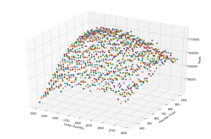
While the overall shape of the values in the grid space is clear, each of the single simulations have a random different color which looks a bit chaotic, see image above.

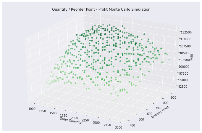
Improved implementation

Therefore I have rearranged the data into an extra designated DataFrame plotdf in order to have the seaborn package access the full series of all profit values, able to sort by value and assign respective color intensity according to their relative value to each other.

So deep green for high profit results and light green for lower. My implementation shows fewer scatter points in the space in comparison to above, this however is only due to time constraints in place even though it has been computer with multiprocessing ;)

from mpl_toolkits.mplot3d import Axes3D

fig = plt.figure(figsize=(12,8))
ax = plt.axes(projection="3d")

plotdf = pd.DataFrame(columns=['q', 'r', 'value'])
for key, val in cc_review_mp.items():
    plotdf.loc[len(plotdf.index)] = [key[0], key[1], val[0]]

ax.scatter3D(xs=plotdf.q, ys=plotdf.r, zs=plotdf.value, marker = 'o', c=plotdf.value, cmap='Greens')

ax.set_xlabel('Order Quantity')
ax.set_ylabel('Reorder Point')
ax.set_zlabel('Profit')
plt.title('Quantity / Reorder Point - Profit Monte Carlo Simulation')
plt.show()

png