Propensity Score Matching on AirAsia Insurance Upsell Data (Causal Inference)
import os
print (os.environ['CONDA_DEFAULT_ENV'])

from platform import python_version

import multiprocessing
!python --version
import platform
print(platform.platform())
print("cpu cores: {0}".format(multiprocessing.cpu_count()))
abtest
Python 3.7.11
Windows-10-10.0.19041-SP0
cpu cores: 12
# Import dependencies
import numpy as np
import pandas as pd
import matplotlib.pyplot as plt
import seaborn as sns
import math
from sklearn.linear_model import LogisticRegression

sns.set_style('darkgrid')
df = pd.read_csv('AncillaryScoring_insurance.csv',encoding='latin-1')
df = df.sample(n=8000).reset_index()
df['index'] = df.index

df.head(3)
| index | Id | PAXCOUNT | SALESCHANNEL | TRIPTYPEDESC | PURCHASELEAD | LENGTHOFSTAY | flight_hour | flight_day | ROUTE | geoNetwork_country | BAGGAGE_CATEGORY | SEAT_CATEGORY | FNB_CATEGORY | INS_FLAG | flightDuration_hour | |
|---|---|---|---|---|---|---|---|---|---|---|---|---|---|---|---|---|
| 0 | 0 | 27345 | 1 | Internet | RoundTrip | 47 | 3 | 4 | Sun | DPSHND | Indonesia | 1 | 0 | 1 | 0 | 7.57 |
| 1 | 1 | 7714 | 1 | Internet | RoundTrip | 2 | 20 | 19 | Fri | DACMEL | Australia | 1 | 0 | 1 | 0 | 8.83 |
| 2 | 2 | 47603 | 1 | Internet | RoundTrip | 37 | 6 | 5 | Sun | ICNSYD | Australia | 0 | 0 | 0 | 0 | 8.58 |
y = df[['INS_FLAG']]
df = df.drop(columns = ['INS_FLAG'])
As this has not been a Randomized Control Experiment there has not really been a flag for control and treatment group. So let’s introduce an artificial treatment effect. Imagine a new booking funnel, a landing page or an advertisement that the customer has been treated with. In our case we convert the variable Seat Category to this treatment indicator.
try:
    df['treatment'] = df.SEAT_CATEGORY
    df = df.drop(columns = ['SEAT_CATEGORY'], axis=1)
except:
    print()
df.info()
<class 'pandas.core.frame.DataFrame'>
RangeIndex: 8000 entries, 0 to 7999
Data columns (total 15 columns):
 #   Column               Non-Null Count  Dtype
---  ------               --------------  -----
 0   index                8000 non-null   int64
 1   Id                   8000 non-null   int64
 2   PAXCOUNT             8000 non-null   int64
 3   SALESCHANNEL         8000 non-null   object
 4   TRIPTYPEDESC         8000 non-null   object
 5   PURCHASELEAD         8000 non-null   int64
 6   LENGTHOFSTAY         8000 non-null   int64
 7   flight_hour          8000 non-null   int64
 8   flight_day           8000 non-null   object
 9   ROUTE                8000 non-null   object
 10  geoNetwork_country   8000 non-null   object
 11  BAGGAGE_CATEGORY     8000 non-null   int64
 12  FNB_CATEGORY         8000 non-null   int64
 13  flightDuration_hour  8000 non-null   float64
 14  treatment            8000 non-null   int64
dtypes: float64(1), int64(9), object(5)
memory usage: 937.6+ KB
There is high correlation between treatment (i.e. hasCabin) and Class. This is desirable in this case as it plays the role of the systematic factor affecting the treatment. In a different context this could be a landing page on site that only specific visitors see.
var = 'BAGGAGE_CATEGORY'
pd.pivot_table(df[['treatment',var,'Id']], \
               values = 'Id', index = 'treatment', columns = var, aggfunc= np.count_nonzero)
| BAGGAGE_CATEGORY | 0 | 1 |
|---|---|---|
| treatment | ||
| 0 | 2221 | 3408 |
| 1 | 454 | 1917 |
df.corr()
| index | Id | PAXCOUNT | PURCHASELEAD | LENGTHOFSTAY | flight_hour | BAGGAGE_CATEGORY | FNB_CATEGORY | flightDuration_hour | treatment | |
|---|---|---|---|---|---|---|---|---|---|---|
| index | 1.000000 | 0.005762 | 0.010263 | 0.012661 | 0.018872 | 0.009092 | 0.000532 | 0.003415 | 0.006561 | 0.004849 |
| Id | 0.005762 | 1.000000 | 0.135480 | 0.015896 | -0.449091 | 0.031731 | -0.174090 | -0.088515 | -0.259993 | -0.000516 |
| PAXCOUNT | 0.010263 | 0.135480 | 1.000000 | 0.208453 | -0.113351 | 0.002100 | 0.117988 | 0.036897 | -0.068885 | 0.035038 |
| PURCHASELEAD | 0.012661 | 0.015896 | 0.208453 | 1.000000 | -0.069222 | 0.037607 | -0.017771 | -0.025227 | 0.072581 | -0.013401 |
| LENGTHOFSTAY | 0.018872 | -0.449091 | -0.113351 | -0.069222 | 1.000000 | -0.023447 | 0.182585 | 0.086383 | 0.141260 | 0.018458 |
| flight_hour | 0.009092 | 0.031731 | 0.002100 | 0.037607 | -0.023447 | 1.000000 | -0.017714 | 0.002793 | -0.008462 | 0.008569 |
| BAGGAGE_CATEGORY | 0.000532 | -0.174090 | 0.117988 | -0.017771 | 0.182585 | -0.017714 | 1.000000 | 0.219758 | 0.051549 | 0.196578 |
| FNB_CATEGORY | 0.003415 | -0.088515 | 0.036897 | -0.025227 | 0.086383 | 0.002793 | 0.219758 | 1.000000 | 0.137707 | 0.310746 |
| flightDuration_hour | 0.006561 | -0.259993 | -0.068885 | 0.072581 | 0.141260 | -0.008462 | 0.051549 | 0.137707 | 1.000000 | 0.097837 |
| treatment | 0.004849 | -0.000516 | 0.035038 | -0.013401 | 0.018458 | 0.008569 | 0.196578 | 0.310746 | 0.097837 | 1.000000 |
Lets get rid of a few variables that do not much lineary correlate with the treatment variable and ideelay keep only those variables that have an affect on the treatment variable.
try:
    df = df.drop(columns = ['PAXCOUNT','PURCHASELEAD','LENGTHOFSTAY','flight_hour'], axis=1)
    df = df.drop(columns = ['ROUTE'], axis=1) # reduce compute resources
except:
    print()
df.info()
df.sample()
<class 'pandas.core.frame.DataFrame'>
RangeIndex: 8000 entries, 0 to 7999
Data columns (total 10 columns):
 #   Column               Non-Null Count  Dtype
---  ------               --------------  -----
 0   index                8000 non-null   int64
 1   Id                   8000 non-null   int64
 2   SALESCHANNEL         8000 non-null   object
 3   TRIPTYPEDESC         8000 non-null   object
 4   flight_day           8000 non-null   object
 5   geoNetwork_country   8000 non-null   object
 6   BAGGAGE_CATEGORY     8000 non-null   int64
 7   FNB_CATEGORY         8000 non-null   int64
 8   flightDuration_hour  8000 non-null   float64
 9   treatment            8000 non-null   int64
dtypes: float64(1), int64(5), object(4)
memory usage: 625.1+ KB
| index | Id | SALESCHANNEL | TRIPTYPEDESC | flight_day | geoNetwork_country | BAGGAGE_CATEGORY | FNB_CATEGORY | flightDuration_hour | treatment | |
|---|---|---|---|---|---|---|---|---|---|---|
| 184 | 184 | 43818 | Mobile | RoundTrip | Sun | Thailand | 1 | 1 | 8.67 | 0 |
Split the treatment variable from the rest of the covariates.
T = df.treatment
X = df.loc[:,df.columns !='treatment']
X.shape
df.shape
T.shape
(8000,)
X_encoded = pd.get_dummies(X, columns = ['SALESCHANNEL', 'TRIPTYPEDESC','flight_day','geoNetwork_country'], \
                           prefix = {'SALESCHANNEL':'sc', 'TRIPTYPEDESC':'tt','flight_day':'fd','geoNetwork_country':'geo'}, drop_first=False)
from sklearn.linear_model import LogisticRegression as lr

from sklearn.pipeline import Pipeline
from sklearn.preprocessing import StandardScaler
from sklearn.neighbors import NearestNeighbors
from sklearn import metrics

# Design pipeline to build the treatment estimator
pipe = Pipeline([
    ('scaler', StandardScaler()),
    ('logistic_classifier', lr())
])

pipe.fit(X_encoded, T)
Pipeline(steps=[('scaler', StandardScaler()),
                ('logistic_classifier', LogisticRegression())])
predictions = pipe.predict_proba(X_encoded)
predictions_binary = pipe.predict(X_encoded)
print('Accuracy: {:.4f}\n'.format(metrics.accuracy_score(T, predictions_binary)))
print('Confusion matrix:\n{}\n'.format(metrics.confusion_matrix(T, predictions_binary)))
print('F1 score is: {:.4f}'.format(metrics.f1_score(T, predictions_binary)))
Accuracy: 0.7315

Confusion matrix:
[[4978  651]
 [1497  874]]

F1 score is: 0.4487
def logit(p):
    logit_value = math.log(p / (1-p))
    return logit_value
Convert propability to logit (based on the suggestion at https://youtu.be/gaUgW7NWai8?t=981)
predictions_logit = np.array([logit(xi) for xi in predictions[:,1]])
# Density distribution of propensity score (logic) broken down by treatment status

sns.set(rc={"figure.figsize":(14, 6)}) #width=8, height=4
fig, ax = plt.subplots(1,2)
fig.suptitle('Density distribution plots for propensity score and logit(propensity score).')
sns.kdeplot(x = predictions[:,1], hue = T , ax = ax[0])
ax[0].set_title('Propensity Score')
sns.kdeplot(x = predictions_logit, hue = T , ax = ax[1])
ax[1].axvline(-0, ls='--')
ax[1].set_title('Logit of Propensity Score')
#ax[1].set_xlim(-5,5)
plt.show()
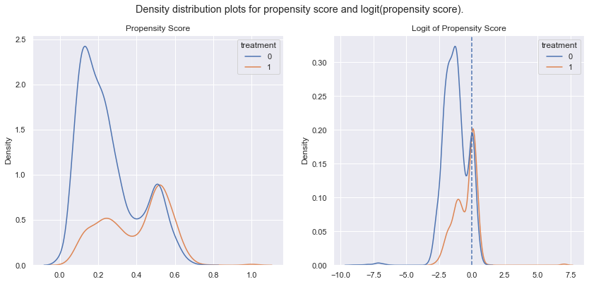
print(max(predictions_logit),min(predictions_logit))
7.120447494606843 -9.159643967495708
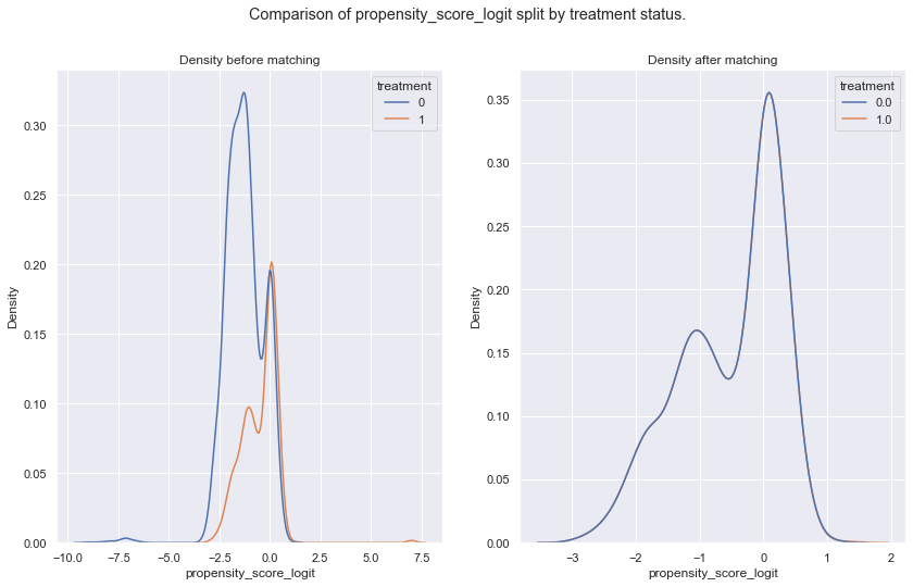
The graph on the right shows the logit propensity scores = the probability distributions of both groups. We can see considerable overlap accross the range of values (-3,2). However on the left of “-3” the probabilities are a lot higher for non the non treatment group as expected. On the right side of zero, this is only marginally true.
For the propensity score matching this overlap is important in order to have balanced matching groups created, this nice overlap will make that work nicely.
print(max(predictions_logit),min(predictions_logit))
common_support = (predictions_logit > -15) & (predictions_logit < 10)
7.120447494606843 -9.159643967495708
df.loc[:,'propensity_score'] = predictions[:,1]
df.loc[:,'propensity_score_logit'] = predictions_logit
df.loc[:,'outcome'] = y.INS_FLAG

X_encoded.loc[:,'propensity_score'] = predictions[:,1]
X_encoded.loc[:,'propensity_score_logit'] = predictions_logit
X_encoded.loc[:,'outcome'] = y.INS_FLAG
X_encoded.loc[:,'treatment'] = df.treatment
Matching Implementation
Use Nearerst Neighbors to identify matching candidates. Then perform 1-to-1 matching by isolating/identifying groups of (T=1,T=0).
- Caliper: 25% of standart deviation of logit(propensity score)
caliper = np.std(df.propensity_score) * 0.25

print('\nCaliper (radius) is: {:.4f}\n'.format(caliper))

df_data = X_encoded

knn = NearestNeighbors(n_neighbors=10 , p = 2, radius=caliper)
knn.fit(df_data[['propensity_score_logit']].to_numpy())
Caliper (radius) is: 0.0427


NearestNeighbors(n_neighbors=10, radius=0.04266206397392259)
For each data point (based on the logit propensity score) obtain (at most) 10 nearest matches. This is regardless of their treatment status.
# Common support distances and indexes
distances , indexes = knn.kneighbors(
    df_data[['propensity_score_logit']].to_numpy(), \
    n_neighbors=10)
print('For item 0, the 4 closest neighbors are (ignore first):')
for ds, idx  in zip(distances[0,0:4], indexes[0,0:4]):
    print('item index: {}'.format(idx))
    print('item distance: {:4f}'.format(ds))
print('...')
For item 0, the 4 closest neighbors are (ignore first):
item index: 0
item distance: 0.000000
item index: 5801
item distance: 0.000156
item index: 4512
item distance: 0.000193
item index: 7128
item distance: 0.000220
...
def propensity_score_matching(row, indexes, df_data):
    current_index = int(row['index']) # index column
    prop_score_logit = row['propensity_score_logit']
    for idx in indexes[current_index,:]:
        if (current_index != idx) and (row.treatment == 1) and (df_data.loc[idx].treatment == 0):
            return int(idx)

df_data['matched_element'] = df_data.reset_index().apply(propensity_score_matching, axis = 1, args = (indexes, df_data))
treated_with_match = ~df_data.matched_element.isna()
treated_matched_data = df_data[treated_with_match][df_data.columns]
treated_matched_data.head(3)
| index | Id | BAGGAGE_CATEGORY | FNB_CATEGORY | flightDuration_hour | sc_Internet | sc_Mobile | tt_CircleTrip | tt_OneWay | tt_RoundTrip | ... | geo_Turkey | geo_United Arab Emirates | geo_United Kingdom | geo_United States | geo_Vietnam | propensity_score | propensity_score_logit | outcome | treatment | matched_element | |
|---|---|---|---|---|---|---|---|---|---|---|---|---|---|---|---|---|---|---|---|---|---|
| 2 | 2 | 10805 | 0 | 1 | 8.83 | 1 | 0 | 0 | 0 | 1 | ... | 0 | 0 | 0 | 0 | 0 | 0.295069 | -0.870892 | 0 | 1 | 3045.0 |
| 8 | 8 | 24136 | 1 | 1 | 8.58 | 1 | 0 | 0 | 0 | 1 | ... | 0 | 0 | 0 | 0 | 0 | 0.562719 | 0.252203 | 0 | 1 | 7051.0 |
| 9 | 9 | 4798 | 1 | 0 | 8.83 | 1 | 0 | 0 | 0 | 1 | ... | 0 | 0 | 0 | 0 | 0 | 0.224072 | -1.242090 | 0 | 1 | 5151.0 |
3 rows × 83 columns
cols = treated_matched_data.columns[0:-1]

def prop_matches(row, data, cols):
    return data.loc[row.matched_element][cols]
%%time

untreated_matched_data = pd.DataFrame(data = treated_matched_data.matched_element)

"""attributes = ['Age', 'SibSp', 'Parch', 'Fare', 'sex_female', 'sex_male', 'embarked_C',
       'embarked_Q', 'embarked_S', 'class_1', 'class_2', 'class_3',
       'propensity_score', 'propensity_score_logit', 'outcome', 'treatment']
"""
for attr in cols:
    untreated_matched_data[attr] = untreated_matched_data.apply(prop_matches, axis = 1, data = df_data, cols = attr)

untreated_matched_data = untreated_matched_data.set_index('matched_element')
untreated_matched_data.head(3)
Wall time: 26.4 s
| index | Id | BAGGAGE_CATEGORY | FNB_CATEGORY | flightDuration_hour | sc_Internet | sc_Mobile | tt_CircleTrip | tt_OneWay | tt_RoundTrip | ... | geo_Thailand | geo_Turkey | geo_United Arab Emirates | geo_United Kingdom | geo_United States | geo_Vietnam | propensity_score | propensity_score_logit | outcome | treatment | |
|---|---|---|---|---|---|---|---|---|---|---|---|---|---|---|---|---|---|---|---|---|---|
| matched_element | |||||||||||||||||||||
| 3045.0 | 3045.0 | 1417.0 | 1.0 | 0.0 | 8.83 | 0.0 | 1.0 | 0.0 | 0.0 | 1.0 | ... | 0.0 | 0.0 | 0.0 | 0.0 | 0.0 | 0.0 | 0.295053 | -0.870966 | 0.0 | 0.0 |
| 7051.0 | 7051.0 | 21235.0 | 1.0 | 1.0 | 8.83 | 1.0 | 0.0 | 0.0 | 0.0 | 1.0 | ... | 0.0 | 0.0 | 0.0 | 0.0 | 0.0 | 0.0 | 0.562535 | 0.251458 | 0.0 | 0.0 |
| 5151.0 | 5151.0 | 23607.0 | 1.0 | 0.0 | 5.62 | 1.0 | 0.0 | 0.0 | 0.0 | 1.0 | ... | 0.0 | 0.0 | 0.0 | 0.0 | 0.0 | 0.0 | 0.224075 | -1.242075 | 0.0 | 0.0 |
3 rows × 82 columns
untreated_matched_data.shape
(2360, 82)
treated_matched_data.shape
(2360, 83)
all_mached_data = pd.concat([treated_matched_data, untreated_matched_data]).reset_index()
all_mached_data.index.is_unique
True
all_mached_data.treatment.value_counts()
1.0    2360
0.0    2360
Name: treatment, dtype: int64
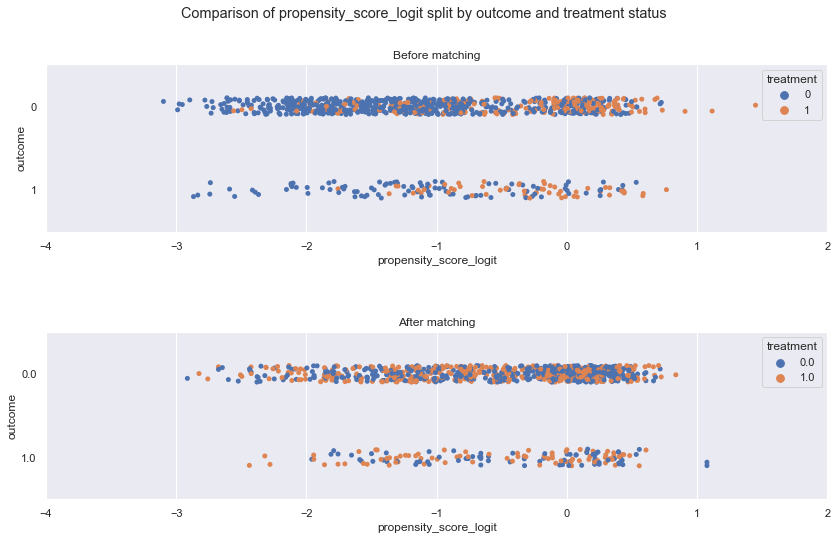
Matching Review
sns.set(rc={"figure.figsize":(14, 8)})
fig, ax = plt.subplots(2,1)
fig.suptitle('Comparison of {} split by outcome and treatment status'.format('propensity_score_logit'))
sns.stripplot(data = df_data.sample(n=1000), y = 'outcome', x = 'propensity_score_logit',
              #alpha=0.7,
              hue = 'treatment', orient = 'h', ax = ax[0]).set(title = 'Before matching', xlim=(-4, 2))
sns.stripplot(data = all_mached_data.sample(n=1000), y = 'outcome', x = 'propensity_score_logit',
              #alpha=0.7,
              hue = 'treatment', ax = ax[1] , orient = 'h').set(title = 'After matching', xlim=(-4, 2))
plt.subplots_adjust(hspace = 0.6)
plt.show()
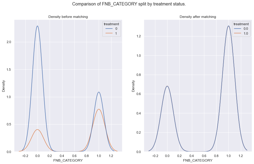
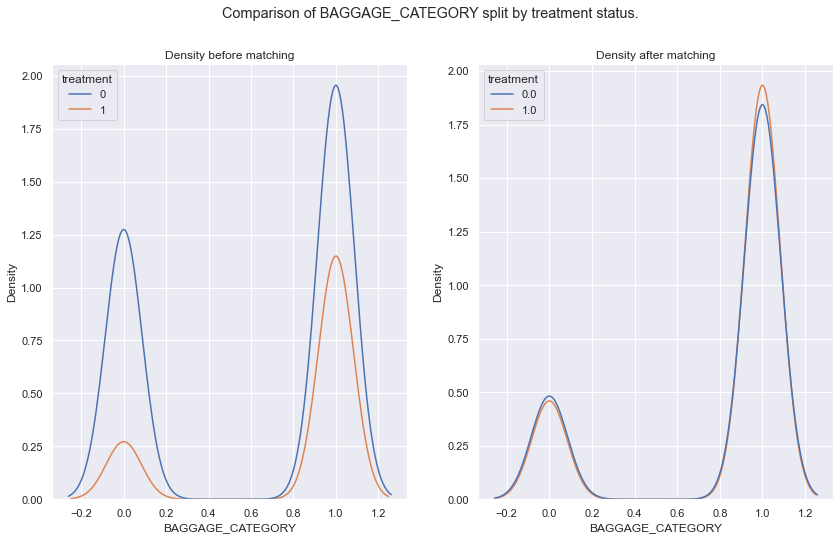
args = ['FNB_CATEGORY','BAGGAGE_CATEGORY','propensity_score_logit']

def plot(arg):
    fig, ax = plt.subplots(1,2)
    fig.suptitle('Comparison of {} split by treatment status.'.format(arg))
    sns.kdeplot(data = df_data, x = arg, hue = 'treatment', ax = ax[0]).set(title='Density before matching')
    sns.kdeplot(data = all_mached_data, x = arg, hue = 'treatment', ax = ax[1]).set(title='Density after matching')
    plt.show()

for arg in args:
    plot(arg)
def cohenD (tmp, metricName):
    treated_metric = tmp[tmp.treatment == 1][metricName]
    untreated_metric = tmp[tmp.treatment == 0][metricName]

    d = ( treated_metric.mean() - untreated_metric.mean() ) / math.sqrt(((treated_metric.count()-1)*treated_metric.std()**2 + (untreated_metric.count()-1)*untreated_metric.std()**2) / (treated_metric.count() + untreated_metric.count()-2))
    return d
%%time
data = []
cols = ['BAGGAGE_CATEGORY', 'FNB_CATEGORY',
'flightDuration_hour', 'sc_Internet', 'sc_Mobile', 'tt_CircleTrip',
'tt_OneWay', 'tt_RoundTrip', 'fd_Fri', 'fd_Mon', 'fd_Sat', 'fd_Sun',
'fd_Thu', 'fd_Tue', 'fd_Wed', 'geo_Vietnam']
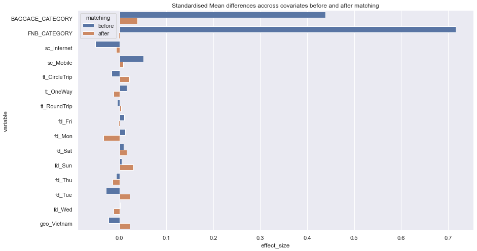
for cl in cols:
data.append([cl,'before', cohenD(df_data,cl)])
data.append([cl,'after', cohenD(all_mached_data,cl)])
Wall time: 78 ms
res = pd.DataFrame(data, columns=['variable','matching','effect_size'])
sn_plot = sns.barplot(data = res, y = 'variable', x = 'effect_size', hue = 'matching', orient='h')
sn_plot.set(title='Standardised Mean differences accross covariates before and after matching')
cols.append('treatment')
Average Treatement effect
overview = all_mached_data[['outcome','treatment']].groupby(by = ['treatment']).aggregate([np.mean, np.var, np.std, 'count'])
print(overview)
            outcome
               mean       var       std count
treatment
0.0        0.138559  0.119411  0.345559  2360
1.0        0.178814  0.146902  0.383277  2360
treated_outcome = overview['outcome']['mean'][1]
treated_counterfactual_outcome = overview['outcome']['mean'][0]
att = treated_outcome - treated_counterfactual_outcome
print('The Average Treatment Effect (ATT): {:.4f}'.format(att))
The Average Treatment Effect (ATT): 0.0403
import warnings
warnings.simplefilter(action='ignore', category=FutureWarning)

from causalinference import CausalModel

# y observed outcome,
# T treatment indicator,
# X covariate matrix (not one hot encoded),
causal = CausalModel(y.values, T, X)
print(causal.summary_stats)
Summary Statistics

                      Controls (N_c=5629)        Treated (N_t=2371)
       Variable         Mean         S.d.         Mean         S.d.     Raw-diff
--------------------------------------------------------------------------------
              Y        0.134        0.341        0.180        0.384        0.045

                      Controls (N_c=5629)        Treated (N_t=2371)
       Variable         Mean         S.d.         Mean         S.d.     Nor-diff
--------------------------------------------------------------------------------
             X0     3992.233     2304.985     4016.753     2320.732        0.011
             X1    25048.731    14472.131    25032.476    14163.444       -0.001
             X2        0.605        0.489        0.809        0.394        0.458
             X3        0.322        0.467        0.658        0.475        0.713
             X4        7.171        1.524        7.493        1.421        0.218
From here we could continue with statistical testing to check if the lift/ treatment effect is significant statistically or we could answer that this minor effect we have noticed is practically not worth the effort and try a better advertisement or landing page.
Conclusion