Monte Carlo Analysis of a Discrete Event Simulation of a non deterministic manufacturing process with multi resources using SimPy
Non-deterministic processes can lead to variability in the response and performance of a system. With our non-determinism in our model, we apply this to characterize how uncertainty propagates through the model. This can be useful in testing the response of our model to different scenarios. This can be helpful in planning future developments and business expansions, conducting stress tests, and preparing for extreme situations.
How can Monte Carlo sampling be used to study processes? We implement a random number generator with the Python random package to generate numbers based on normal distributions. The real goal of using Monte Carlo sampling in discrete-event models is to study model uncertainty arising from nondeterministic processes. In other words, this can help characterize uncertainty to support specific management decisions.
As we have seen, uncertainty propagates through a system at each process duration, leading to different model trajectories, often referred to as response envelopes. In our manufacturing process, there are nine process activities that are defined in a large dictionary and visualized below.

We use a terminating type of simulation where we predefine the length of the simulation beforehand. In our case a work week of 6 work days, with 24 hours and 60 mins each resulting in 8640 mins of simulation time (6 * 24 * 60).
In that work week the manufacturer has a minimum goal of producing 10% more than the regular 160 batches on the given production line. Besides the given capacity configuration two additional capacities configurations (vectors) are to be examined
1. [1,1,1,1,1,1,2,1,1], baseline
2. [2,1,1,1,1,1,2,1,1], bottleneck 'raw material goods receipt' increased by one (Scenario 1)
3. [2,1,1,1,1,1,3,1,1]. 'Raw material goods receipt' and 'Final Assembly' increased each by one (Scenario 2)
Statistical Analysis included
A simulation is a computer-based statistical sampling experiment. Therefore, we need statistical techniques to analyze simulation experiments.
We will resort to the central limit theorem (C.L.T.) to deal with the simulation data. It states that the distribution of a sample mean approaches a normal distribution where the mean is equal to the population mean and the variance is equal to sigma squared/n, where sigma squared is the population variance and n is the number of observations in the data.
We will also calculate confidence intervals (CI) in order to deal with errors in the sample means. Based on the central limit theorem, such a confidence interval indicates the magnitude of this error.
Simulation with SimPy
A machining production line of nine process activities is subject to our simulation. Arrivals are Poisson distributed and occur at a mean rate of 1 batch every 45 mins. The machining process consists of 9 activities with each are modeled as a resource itself meaning the equipment and manpower at the same time. The processing time for each activity is assumed to be normally distributed and each mean and standard distribution is estimated respectively. The exception is a unified distributed activity ‘Packaging’ for the sake of demonstration. The shop schedules batches on FIFO (First In, First Out) policy.
The owners of the company plan to make certain improvements to increase the company’s production. As a first step, they decide to conduct a simulation study of the current system, obtain some measures of performance, and then compare them with those of a proposed improvement.
Analysis
The company’s owners are interested in the short-term behavior of the system. The shop has a weekly predictable demand, so they decided to use six work days 62460 = 8640 minutes of simulated time as the terminal event.
For the initial conditions, the model starts with all activities idle but with a job ready to start (inital_delay = 0).
Once the probability distributions of the arrivals and services have been identified and the initial conditions have been established, it is essential to perform a data verification process to check that the model coding is correct and to detect programming errors before proceeding with production runs. I have done that with value changes and tracing through print statements.
import random
import simpy
import matplotlib.pyplot as plt
import numpy as np
import pandas as pd
import seaborn as sns
import schemdraw
from schemdraw.flow import *
def print_stats(res):
    """Simpy native function to allow looking into queues and resource utilization while the simulation runs"""
    print(f'{res.count} of {res.capacity} slots are allocated.')
    print(f'  Users: {res.users}')
    print(f'  Queued events: {res.queue}')
    print(f'\n')

def all_processes(env, batch_i, verbose=True):
    """Modeling the whole manufacturing process that is defined in the process_activities dictionary by scheduling, processing
    and releasing batches from/to resources"""

    for p_activity in process_activities:

        if verbose==True:
            print("> New production batch " + str(batch_i) + " scheduled for " +
                  p_activity.get('Name') + "@ current time: " + str(np.round(env.now, 2)))

        resource = p_activity.get('Resource')
        request_time = env.now

        resource_request = resource.request()

        batch_activity_df.loc[(batch_i, p_activity.get('Name')), 'Scheduled'] = env.now

        yield resource_request

        if verbose==True:
            print("> Start processing batch " + str(batch_i) + " scheduled for " +
                  p_activity.get('Name') + " @current time: " + str(np.round(env.now, 2)))

        batch_activity_df.loc[(batch_i, p_activity.get('Name')), 'Processing'] = env.now

        duration = activity(gen_type=p_activity.get('gen_type'),
                                       gauss_mean=p_activity.get('Average_Duration'),
                                       gauss_std=p_activity.get('Standard_Deviation'),
                                       unif_start=p_activity.get('Start_Range'),
                                       unif_end=p_activity.get('End_Range')
                           )

        if (env.now > request_time):
            if verbose==True:
                print("batch {} had to wait " + str(np.round(env.now - request_time,2)) + " mins on activity {}".format(batch_i,
                                                                            p_activity.get('Name')))
            batch_activity_df.loc[(batch_i, p_activity.get('Name')), 'Wait_time'] = env.now - request_time
        try:
            yield env.timeout(duration)
        except: # negative durations may occur due to erroneous distributions
            print(duration, p_activity.get('Name'))

        resource.release(resource_request)
        batch_activity_df.loc[(batch_i, p_activity.get('Name')), 'Releasing'] = env.now
        if verbose==True:
            print("> Finished Batch " + str(batch_i) + " processed on activity " +
                  p_activity.get('Name') + " in " + str(np.round(duration,2))
                  + " minutes => current time: " + str(np.round(env.now, 2)))
def activity(gen_type=None, gauss_mean=None, gauss_std=None, unif_start=None, unif_end=None):
    """Minor process activity property helper function"""
    if gen_type == "gauss":
        duration = random.gauss(gauss_mean, gauss_std)
    elif gen_type == "uniform":
        duration = random.uniform(unif_start, unif_end)
    return duration


def batch_generator(env, verbose=True):
    """Manufacturing Batch generation with batch seeded Poisson distributed arrival times"""
    batch_i = 0

    while True:

        inter_arrival_time = np.random.default_rng(batch_i).poisson(45, 1)

        yield env.timeout(inter_arrival_time)
        if verbose==True:
            print('new batch generated: ', batch_i)
        env.process(all_processes(env, batch_i, verbose=verbose))
        batch_i += 1
#rng = np.random.default_rng()
#plt.hist(rng.poisson(45, 1))
global performance_series
performance_df = pd.DataFrame(columns = ['num_complete_batches', 'capacity_vector'])


global utilization_df
utilization_df = pd.DataFrame(columns = ['Raw Material Goods receipt',
                                         'Pre-Cutting',
                                         'Polishing',
                                         'Adding Component 1',
                                         'Adding Component 2',
                                         'Adding Component 3',
                                         'Final assembly',
                                         'Quality control',
                                         'Packaging', 'capacity_vector'])
global error_check
error_check = pd.DataFrame(columns = ['Raw Material Goods receipt',
                                         'Pre-Cutting',
                                         'Polishing',
                                         'Adding Component 1',
                                         'Adding Component 2',
                                         'Adding Component 3',
                                         'Final assembly',
                                         'Quality control',
                                         'Packaging'])

global batch_cycle_time_df
batch_cycle_time_df = pd.DataFrame(columns = ['run_id', 'batch_id', 'process_cycle_time', 'capacity_vector'])

global wait_time_df
wait_time_df = pd.DataFrame(columns = ['activity', 'mean', 'run_id', 'capacity_vector'])

def run_monte_carlo(capacity_vector):
    """Conducting Monte Carlo simulation runs with a given capacity vector of the defined process in the
    process_activities dict implemented with Simpy Simulation Framework"""
    run_i = 0
    runs = 50

    while run_i < runs:
    #for run_i in range(runs):

        random.seed(run_i)

        env = simpy.Environment()

        global process_activities
        process_activities = [{'Name': 'Raw Material Goods receipt',
                               'gen_type': "gauss",
          'Average_Duration': 50,
          'Standard_Deviation': 5,
          'Resource': simpy.Resource(env, capacity=capacity_vector[0])},

         {'Name': 'Pre-Cutting', 'gen_type': "gauss",
          'Average_Duration': 20,
          'Standard_Deviation': 3,
          'Resource': simpy.Resource(env, capacity=capacity_vector[1])},

         {'Name': 'Polishing', 'gen_type': "gauss",
          'Average_Duration': 20,
          'Standard_Deviation': 5,
          'Resource': simpy.Resource(env, capacity=capacity_vector[2])},

         {'Name': 'Adding Component 1', 'gen_type': "gauss",
          'Average_Duration': 5,
          'Standard_Deviation': 1,
          'Resource': simpy.Resource(env, capacity=capacity_vector[3])},

         {'Name': 'Adding Component 2', 'gen_type': "gauss",
          'Average_Duration': 10,
          'Standard_Deviation': 2,
          'Resource': simpy.Resource(env, capacity=capacity_vector[4])},

         {'Name': 'Adding Component 3', 'gen_type': "gauss",
          'Average_Duration': 8,
          'Standard_Deviation': 1,
          'Resource': simpy.Resource(env, capacity=capacity_vector[5])},

         {'Name': 'Final assembly', 'gen_type': "gauss",
          'Average_Duration': 90,
          'Standard_Deviation': 10,
          'Resource': simpy.Resource(env, capacity=capacity_vector[6])},

         {'Name': 'Quality control', 'gen_type': "gauss",
          'Average_Duration': 10,
          'Standard_Deviation': 1,
          'Resource': simpy.Resource(env, capacity=capacity_vector[7])},

         {'Name': 'Packaging', 'gen_type': "uniform",
          'Start_Range': 5,
          'End_Range': 10,
          'Resource': simpy.Resource(env, capacity=capacity_vector[8])}
        ]

        global batch_activity_df
        batch_activity_df = pd.DataFrame(columns = ['batchid', 'activity', 'Scheduled',
                                            'Processing', 'Releasing', 'Wait_time']).set_index(['batchid', 'activity'])

        #six day week
        #duration in mins
        sim_duration = 6*24*60

        b = env.process(batch_generator(env, verbose=False))
        c = env.run(until=sim_duration)

        process_stats(batch_activity_df, capacity_vector, sim_duration, run_i)

        # wait times stats across activities
        #wait_time_stats_list.append(pd.pivot_table(data=batch_activity_df, index=['activity'],
        #       aggfunc=['min', 'max', 'mean', 'median', 'sum'], values='Wait_time',
        #       fill_value=0
        #      ))

        print('monte carlo run: ' + str(run_i))
        run_i += 1

        #del env
        #del b
        #del c
def process_stats(batch_activity_df, capacity_vector, sim_duration, run_i):
    """Processing stats for each sim run for later analysis"""

    ba_df = batch_activity_df.copy(deep=True)
    ba_df['Releasing'].fillna(sim_duration, inplace=True)
    ba_df['Processing_duration'] = ba_df.Releasing - ba_df.Processing
    process_durations_series = ba_df.groupby('activity')['Processing_duration'].sum()

    #check
    caps = np.multiply(capacity_vector, sim_duration)
    #print(capacity_vector)
    #print(process_durations_series)

    # activity durations
    process_durations_df = pd.DataFrame(data=[process_durations_series,
                                          pd.Series(np.multiply(capacity_vector, sim_duration),
                                                    name='Capacity',
                                                    index=list((object['Name'] for object in process_activities)))],
                                   ).T

    if len(process_durations_df.Capacity) == len(process_durations_series):
        process_durations_df['Utilization_perc'] = np.round(process_durations_df.Processing_duration.astype(float).divide(process_durations_df.Capacity.astype(float))*100,2)
    else:
        print('lengths: ', len(process_durations_df.Capacity), len(process_durations_series))

    #error check
    error_check.loc[run_i] = process_durations_series

    # resource utilization
    #print(type(process_durations_df['Utilization_perc']))
    util = process_durations_df['Utilization_perc'].copy()
    util['capacity_vector'] = str(capacity_vector)
    #display(util)
    utilization_df.loc[len(utilization_df)] = util

    # performance
    # count complete batches
    # must use untouched batch_activity_df!
    # max batch_id + 1 for the count
    max_compl_batch = batch_activity_df.loc[(slice(None), 'Packaging'), ['Scheduled','Processing','Releasing']].sort_values('batchid', ascending=False).dropna(how='any').index.max()[0]

    performance_df.loc[len(performance_df)] = [max_compl_batch+1, str(capacity_vector)]

    # wait_time

    wt_df = batch_activity_df.copy().reset_index()
    compl_batches_df = wt_df.loc[wt_df['batchid'] <= max_compl_batch]
    #compl_batches_df = batch_activity_df.query('0 <= batchid <='+ str(max_compl_batch))
    run_activity_mean_wait_time_df = pd.pivot_table(data=compl_batches_df, index=['activity'],
                                       aggfunc=['mean'], values='Wait_time',
                                       fill_value=0)
    run_activity_mean_wait_time_df['run_id'] = run_i
    run_activity_mean_wait_time_df['capacity_vector'] = str(capacity_vector)
    run_activity_mean_wait_time_df.columns = run_activity_mean_wait_time_df.columns.droplevel(1)
    run_activity_mean_wait_time_df.reset_index(inplace=True)
    #print(run_activity_mean_wait_time_df)
    global wait_time_df
    wait_time_df = pd.concat([wait_time_df, run_activity_mean_wait_time_df])

    # process cycle time
    # must use untouched batch_activity_df!
    for batch_id in range(max_compl_batch+1):
        start = float(batch_activity_df.loc[(batch_id, 'Raw Material Goods receipt'), ['Processing']])
        end = float(batch_activity_df.loc[(batch_id, 'Packaging'), ['Releasing']])
        process_cycle_time = end - start
        batch_cycle_time_df.loc[len(batch_cycle_time_df)] = [run_i, batch_id, float(process_cycle_time), str(capacity_vector)]
#run_monte_carlo([1,1,1,1,1,1,2,1,1])
capacity_vectors = [
                    [1,1,1,1,1,1,2,1,1],
                    [2,1,1,1,1,1,2,1,1],
                    [2,1,1,1,1,1,3,1,1]
                   ]

# Call the run_monte_carlo function across all capacities scenarios in form of capacity vectors
for capacity_vector in capacity_vectors:
    run_monte_carlo(capacity_vector)
performance_df
| num_complete_batches | capacity_vector | |
|---|---|---|
| 0 | 167 | [1, 1, 1, 1, 1, 1, 2, 1, 1] |
| 1 | 168 | [1, 1, 1, 1, 1, 1, 2, 1, 1] |
| 2 | 167 | [1, 1, 1, 1, 1, 1, 2, 1, 1] |
| 3 | 167 | [1, 1, 1, 1, 1, 1, 2, 1, 1] |
| 4 | 167 | [1, 1, 1, 1, 1, 1, 2, 1, 1] |
| ... | ... | ... |
| 145 | 186 | [2, 1, 1, 1, 1, 1, 3, 1, 1] |
| 146 | 186 | [2, 1, 1, 1, 1, 1, 3, 1, 1] |
| 147 | 186 | [2, 1, 1, 1, 1, 1, 3, 1, 1] |
| 148 | 186 | [2, 1, 1, 1, 1, 1, 3, 1, 1] |
| 149 | 185 | [2, 1, 1, 1, 1, 1, 3, 1, 1] |
150 rows × 2 columns
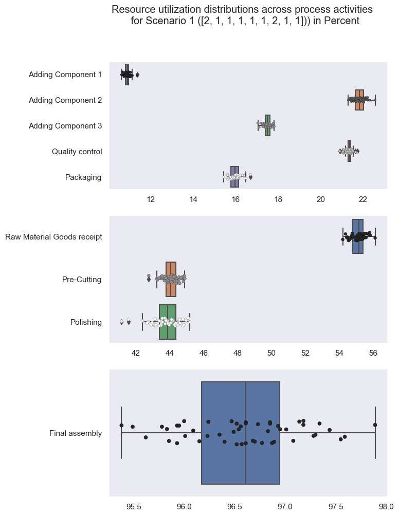
Displaying a few insights into resource utilization distributions across process activities for Scenario 1.
set1 = ['Adding Component 1', 'Adding Component 2', 'Adding Component 3', 'Quality control', 'Packaging', 'capacity_vector']
set2 = ['Raw Material Goods receipt', 'Pre-Cutting','Polishing']
set3 = ['Final assembly', 'capacity_vector']

utilization_df2 = utilization_df[utilization_df['capacity_vector'] == '[2, 1, 1, 1, 1, 1, 2, 1, 1]'].copy()

fig, axs = plt.subplots(3, figsize=(7, 11))
fig.suptitle('Resource utilization distributions across process activities \n for Scenario 1 ([2, 1, 1, 1, 1, 1, 2, 1, 1])) in Percent')

sns.boxplot(data=utilization_df2[set1], orient='h', ax=axs[0])
sns.stripplot(data=utilization_df2[set1], orient='h',size=3, palette='dark:white', linewidth=0.5, ax=axs[0], #hue='capacity_vector'
             )

sns.boxplot(data=utilization_df2[set2], orient='h', ax=axs[1])
sns.stripplot(data=utilization_df2[set2], orient='h',size=4,  palette='dark:white', linewidth=0.5, ax=axs[1])

sns.boxplot(data=utilization_df2[set3], orient='h')
sns.stripplot(data=utilization_df2[set3], orient='h',size=5,  palette='dark:white', linewidth=0.5, ax=axs[2])

plt.show()
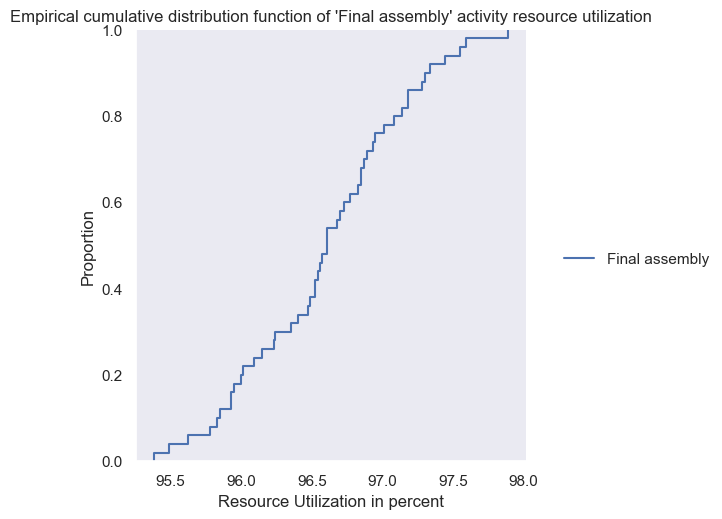
sns.displot(data=utilization_df2[set3], kind="ecdf")
plt.title("Empirical cumulative distribution function of 'Final assembly' activity resource utilization")
plt.xlabel('Resource Utilization in percent')
plt.show()
def pdf(performance_df):
    """Analyse and visualize performance stats ex post across runs"""
    pivot = pd.pivot_table(data=performance_df, index=['capacity_vector'],
               aggfunc=[ 'count', 'mean', 'sem']
                        ,# values='num_complete_batches',
               #fill_value=0
              ).droplevel(1, axis=1)

    df = pivot.copy()

    from scipy import stats
    confidence = 0.90
    dof = len(df)-1
    critical_val_z = np.abs(stats.t.ppf((1-confidence)/2,dof))

    df['ci_upper_limit'] = df['mean'] + critical_val_z * df['sem']
    df['ci_lower_limit'] = df['mean'] - critical_val_z * df['sem']
    df['performance_index_percent'] = np.round(df['mean'] / df['mean'].min() *100, 2)

    title = 'Performance Comparison for two new capacity configurations vs. baseline (completed batches per work week)'
    print(title)
    display(df)

    sns.set(rc={'figure.figsize':(6,9)})
    sns.set_style('dark')
    sns.barplot(data=performance_df, y='num_complete_batches', x='capacity_vector', errorbar=('ci', 90))
    plt.title(title)
    plt.ylabel('Average Number of completed batches')
    plt.xlabel('Capacity configurations as vectors')
    plt.show()
We made 50 independent replications for each capacity configuration. As previously indicated, the independence of each run is accomplished by using unique seeds of random numbers in each run to accomplish the statistical independence across runs.
The table the sample means, the sample standard deviations, and the lower and upper bounds of the confidence intervals. We can claim with approximately 90% confidence that the process performance with baseline capacity is within [167.995327, 167.004673] batches for example.
The interval confidence is in all cases quite low to be sufficiently confident about the performance differences as all confidence intervals do not overlap each other.
pdf(performance_df)
Performance Comparison for two new capacity configurations vs. baseline (completed batches per work week)
| count | mean | sem | ci_upper_limit | ci_lower_limit | performance_index_percent | |
|---|---|---|---|---|---|---|
| capacity_vector | ||||||
| [1, 1, 1, 1, 1, 1, 2, 1, 1] | 50 | 167.50 | 0.169633 | 167.995327 | 167.004673 | 100.00 |
| [2, 1, 1, 1, 1, 1, 2, 1, 1] | 50 | 184.28 | 0.117942 | 184.624388 | 183.935612 | 110.02 |
| [2, 1, 1, 1, 1, 1, 3, 1, 1] | 50 | 185.98 | 0.034876 | 186.081837 | 185.878163 | 111.03 |
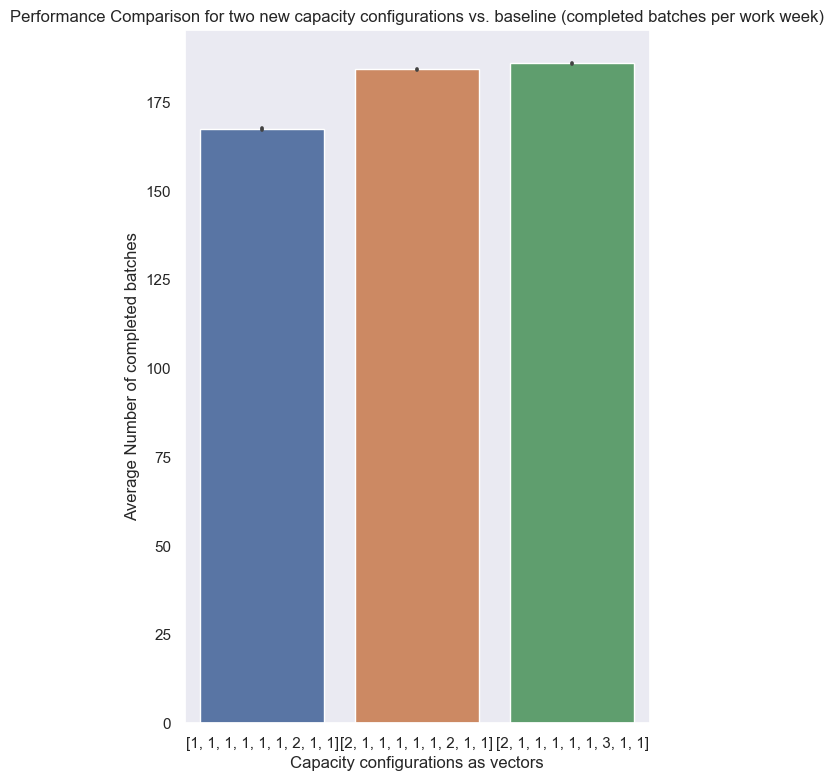
While the initial capacity increase in the ‘Raw Material Goods receipt’ activity helped to alleviate the apparent bottleneck there the performance could be lifted by round about 10% towards a mean of 183.28 batches per work week with a quite low variance.
However increasing the capacity of the second bottleneck in line with ‘Final assembly’ in a second Scenario does not prove to be equally lifting performance. The simple reason for that is the fact is that the mere performance is now limited by its predecessing process: the current rate of batch deliveries disallow further gains as the table of mean wait times per capacity vector shows us below. While the initial baseline had a significant mean wait time the first and second capacity scenarios diminished queues and wait times tremendously.
try:
    wait_time_df['mean'] = wait_time_df['mean'].str[0]
except:
    pass

wait_time_df.groupby('capacity_vector').mean()
| mean | |
|---|---|
| capacity_vector | |
| [1, 1, 1, 1, 1, 1, 2, 1, 1] | 135.426018 |
| [2, 1, 1, 1, 1, 1, 2, 1, 1] | 11.136825 |
| [2, 1, 1, 1, 1, 1, 3, 1, 1] | 4.014474 |
We can see the signifcantly different trajectories of the various capacity models and how its variations in the process performances reflect in process cycle times. The model response envelope spans from batches finishing as low as about 180 mins up to 400 mins when bottlenecks are encountered.
pd.pivot_table(data=batch_cycle_time_df, index=['capacity_vector'],
               aggfunc=['min', 'max', np.mean, 'median', 'sum'], values='process_cycle_time')
| min | max | mean | median | sum | |
|---|---|---|---|---|---|
| process_cycle_time | process_cycle_time | process_cycle_time | process_cycle_time | process_cycle_time | |
| capacity_vector | |||||
| [1, 1, 1, 1, 1, 1, 2, 1, 1] | 173.525406 | 344.863612 | 224.257911 | 224.171241 | 1.878160e+06 |
| [2, 1, 1, 1, 1, 1, 2, 1, 1] | 178.650044 | 426.589912 | 259.831559 | 253.852942 | 2.393828e+06 |
| [2, 1, 1, 1, 1, 1, 3, 1, 1] | 169.809370 | 275.000000 | 220.786957 | 220.624455 | 2.053098e+06 |
batch_cycle_time_df.sort_values('process_cycle_time', ascending=False)
| run_id | batch_id | process_cycle_time | capacity_vector | |
|---|---|---|---|---|
| 9470 | 5 | 172 | 426.589912 | [2, 1, 1, 1, 1, 1, 2, 1, 1] |
| 9468 | 5 | 170 | 411.855372 | [2, 1, 1, 1, 1, 1, 2, 1, 1] |
| 9471 | 5 | 173 | 411.139876 | [2, 1, 1, 1, 1, 1, 2, 1, 1] |
| 9288 | 4 | 173 | 403.481199 | [2, 1, 1, 1, 1, 1, 2, 1, 1] |
| 9472 | 5 | 174 | 401.780125 | [2, 1, 1, 1, 1, 1, 2, 1, 1] |
| ... | ... | ... | ... | ... |
| 26361 | 47 | 30 | 174.235950 | [2, 1, 1, 1, 1, 1, 3, 1, 1] |
| 6764 | 40 | 62 | 173.525406 | [1, 1, 1, 1, 1, 1, 2, 1, 1] |
| 20423 | 15 | 44 | 172.842086 | [2, 1, 1, 1, 1, 1, 3, 1, 1] |
| 20250 | 14 | 57 | 169.809370 | [2, 1, 1, 1, 1, 1, 3, 1, 1] |
| 15554 | 38 | 183 | NaN | [2, 1, 1, 1, 1, 1, 2, 1, 1] |
26888 rows × 4 columns
# appendix
# just visualizing the process

fontsize=11
boxwidth=2.5
counter=0
schemdraw.theme(theme='dark')

with schemdraw.Drawing() as d:
    d+= Start().label('Start', fontsize=fontsize)
    d+= Arrow().right(d.unit)

    for p_activity in process_activities:
        name = p_activity.get('Name')

        d+= Box(w = boxwidth).label(p_activity.get('Name').replace(" ","\n"), fontsize=fontsize)
        if counter < 3:
            d+= Arrow().right(d.unit/2)
        elif counter == 3:
            d+= Arrow().down(d.unit/2)
        elif counter == 4:
            d+= Arrow().left(d.unit)
        else:
            d+= Arrow().left(d.unit/2)
        counter += 1

    #End program
    d+= (end := Ellipse().label("End", fontsize=fontsize))
d.save('process_schemadraw.svg')