Bayes Theorem applied in Python incl. A/B Testing example - Notes
| \ | Frequentist (classical) approach | Bayesian approach |
|---|---|---|
| probability | proportion of outcomes | degree of belief |
| parameters | fixed values/constants | random variables |
| names | confidence interval, p-value, power, significance | credible interval, prior, posterior |
$\Large P(A\mid B)= \frac{P(B\mid A)P(A)}{P(B)}$
$\ P(A\mid B) = Posterior $
$\ P(B\mid A) = Likelihood $
$\ P(A) = Prior $
$\ P(B) = Evidence :(=scaling factor)$
Bayesian estimation
grid approximation
import numpy as np
import pandas as pd
from scipy.stats import uniform, binom

import matplotlib.pyplot as plt
import seaborn as sns
sns.set_style("darkgrid")
# Create cured patients array from 1 to 10
num_patients_cured = np.arange(0,11)

# Create efficacy rate array from 0 to 1 by 0.01
efficacy_rate = np.arange(0,1.01, 0.01)

# Combine the two arrays in one DataFrame
df = pd.DataFrame([(x, y) for x in num_patients_cured for y in efficacy_rate])

# Name the columns
df.columns = ["num_patients_cured", "efficacy_rate"]

# Print df
print(df)
      num_patients_cured  efficacy_rate
0                      0           0.00
1                      0           0.01
2                      0           0.02
3                      0           0.03
4                      0           0.04
...                  ...            ...
1106                  10           0.96
1107                  10           0.97
1108                  10           0.98
1109                  10           0.99
1110                  10           1.00

[1111 rows x 2 columns]
grid approximation without prior knowledge - prior is uniform distribution
# Calculate the prior efficacy rate and the likelihood
df["prior"] = uniform.pdf(df["efficacy_rate"])
df["likelihood"] = binom.pmf(df["num_patients_cured"], 10, df["efficacy_rate"])
# Calculate the posterior efficacy rate and scale it to sum up to one
df["posterior_prob"] = df["prior"] * df["likelihood"]
df["posterior_prob"] /= df["posterior_prob"].sum()
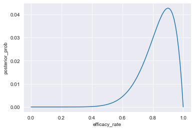
# Compute the posterior probability of observing 9 cured patients
df_9_of_10_cured = df.loc[df["num_patients_cured"] == 9].copy()
df_9_of_10_cured["posterior_prob"] /= df_9_of_10_cured["posterior_prob"].sum()
# Plot the drug's posterior efficacy rate having seen 9 out of 10 patients cured.
sns.set_style("darkgrid")
sns.lineplot(x=df_9_of_10_cured["efficacy_rate"], y=df_9_of_10_cured["posterior_prob"] )
plt.show()
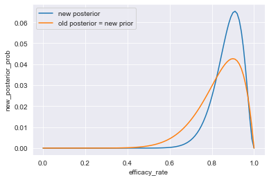
The testing of the drug continues, and a group of additional 12 sick patients have been treated, 10 of whom were cured.
Updating the posterior belief: as prior the previous posterior probability is used
# Assign old posterior to new prior and calculate likelihood
df["new_prior"] = df["posterior_prob"]
df["new_likelihood"] = binom.pmf(df["num_patients_cured"], 12, df["efficacy_rate"])

# Calculate new posterior and scale it
df["new_posterior_prob"] = df["new_prior"] * df["new_likelihood"]
df["new_posterior_prob"] /= df["new_posterior_prob"].sum()

# Compute the posterior probability of observing 10 cured patients
df_10_of_12_cured = df[df["num_patients_cured"] == 10].copy()
df_10_of_12_cured["new_posterior_prob"] /= df_10_of_12_cured["new_posterior_prob"].sum()

sns.lineplot(x=df_10_of_12_cured["efficacy_rate"],
             y=df_10_of_12_cured["new_posterior_prob"],
             label="new posterior")
sns.lineplot(x=df_9_of_10_cured["efficacy_rate"],
             y=df_9_of_10_cured["posterior_prob"],
             label="old posterior = new prior")
plt.show()
# compare old and new likelihood
data = {
    'likelihood': binom.pmf(df["num_patients_cured"], 10, df["efficacy_rate"])[0:10],
    'new likelihood': binom.pmf(df["num_patients_cured"], 12, df["efficacy_rate"])[0:10]
}

pd.DataFrame(data=data)
| likelihood | new likelihood | |
|---|---|---|
| 0 | 1.000000 | 1.000000 |
| 1 | 0.904382 | 0.886385 |
| 2 | 0.817073 | 0.784717 |
| 3 | 0.737424 | 0.693842 |
| 4 | 0.664833 | 0.612710 |
| 5 | 0.598737 | 0.540360 |
| 6 | 0.538615 | 0.475920 |
| 7 | 0.483982 | 0.418596 |
| 8 | 0.434388 | 0.367666 |
| 9 | 0.389416 | 0.322475 |
binom.pmf(df["num_patients_cured"], 12, df["efficacy_rate"])
array([1.        , 0.88638487, 0.78471672, ..., 0.02157072, 0.00596892,
       0.        ])
Prior distribution
= chosen and stated before we see the data (no cherry picking)
can be
- old prior
- expert opinion
- common knowledge
- previous research
- subjective belief
conjugate priors
= Some priors,multiplied with specic likelihoods, yield known posteriors
for example:
# prior: Beta(a, b)
# posterior: Beta(x, y)
# with
# x = NumberOfSuccesses + a
# y = NumberOfObservations - NumberOfSuccesses + b
Two methods to get the posterior
Simulation
draws = np.random.beta(2,4,1000)
draws[0:10]
array([0.24647378, 0.11933372, 0.38872732, 0.4030806 , 0.59654602,
       0.01687355, 0.29056646, 0.14239311, 0.17596316, 0.5461129 ])
#sns.kdeplot(draws)
Calculation
if posterior not know we can calculate using grid approximation
#sns.lineplot(x=df["efficacy_rate"], y=df["posterior_prob"] )
df.head()
| num_patients_cured | efficacy_rate | prior | likelihood | posterior_prob | new_prior | new_likelihood | new_posterior_prob | |
|---|---|---|---|---|---|---|---|---|
| 0 | 0 | 0.00 | 1.0 | 1.000000 | 0.009901 | 0.009901 | 1.000000 | 0.050946 |
| 1 | 0 | 0.01 | 1.0 | 0.904382 | 0.008954 | 0.008954 | 0.886385 | 0.040840 |
| 2 | 0 | 0.02 | 1.0 | 0.817073 | 0.008090 | 0.008090 | 0.784717 | 0.032665 |
| 3 | 0 | 0.03 | 1.0 | 0.737424 | 0.007301 | 0.007301 | 0.693842 | 0.026067 |
| 4 | 0 | 0.04 | 1.0 | 0.664833 | 0.006583 | 0.006583 | 0.612710 | 0.020753 |
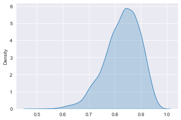
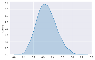
Simulating posterior draws
Beta(5, 2) prior
# Define the number of patients treated and cured
num_patients_treated = 22
num_patients_cured = 19

# Simulate 10000 draws from the posterior distribution
posterior_draws = np.random.beta(num_patients_cured + 5, num_patients_treated - num_patients_cured + 2, 10000)

# Plot the posterior distribution
sns.kdeplot(data=posterior_draws, shade=True)
plt.show()
Reporting Bayesian results
sometimes information on distributions needs to be condensed and single number of a parameter is needed
point estimates
- mean
- median
- credible interval (vs. confidence interval [frequentist])
credible interval
the credible interval is the probability that the parameter falls inside credible interval bounds (vs. confidence interval [frequentist])
# Calculate the expected number of people cured
cured_expected = np.mean(posterior_draws) * 100_000 # 100k infections

# Calculate the minimum number of people cured with 50% probability
min_cured_50_perc = np.median(posterior_draws) * 100_000

# Calculate the minimum number of people cured with 90% probability
min_cured_90_perc = np.percentile(posterior_draws, 10) * 100000

# Print the filled-in memo
print(f"Based on the experiments carried out by ourselves and neighboring countries, \nshould we distribute the drug, we can expect {int(cured_expected)} infected people to be cured. \nThere is a 50% probability the number of cured infections \nwill amount to at least {int(min_cured_50_perc)}, and with 90% probability \nit will not be less than {int(min_cured_90_perc)}.")
Based on the experiments carried out by ourselves and neighboring countries,
should we distribute the drug, we can expect 82798 infected people to be cured.
There is a 50% probability the number of cured infections
will amount to at least 83550, and with 90% probability
it will not be less than 73539.
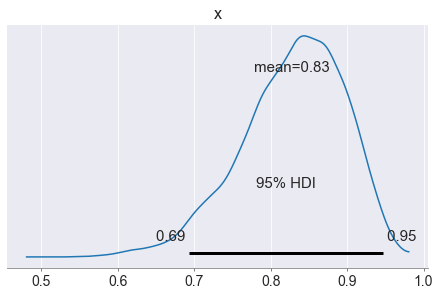
Highest Posterior Density (HPD)
to calculate the credible intervals, as the low and high bounds in which the parameter lies with X% probability
# Import pymc3 as pm
import pymc3 as pm
# hpd function deprecated
# using hdi (highest density interval) instead

ci_67 = pm.hdi(posterior_draws, hdi_prob=0.67)
#print(ci_67)

# Calculate HPD credible interval of 90%
ci_90 = pm.hdi(posterior_draws, hdi_prob=0.9)

# Calculate HPD credible interval of 95%
ci_95 = pm.hdi(posterior_draws, hdi_prob=0.95)

pm.plot_posterior(np.array(posterior_draws), hdi_prob=0.95)
# Print the memo
print(f"The experimental results indicate that with a 90% probability \nthe new drug's efficacy rate is between {np.round(ci_90[0], 2)} and {np.round(ci_90[1], 2)}, \nand with a 95% probability it is between {np.round(ci_95[0], 2)} and {np.round(ci_95[1], 2)}.")
The experimental results indicate that with a 90% probability
the new drug's efficacy rate is between 0.72 and 0.94,
and with a 95% probability it is between 0.69 and 0.95.
Bayesian inference
A/B testing
# 1 heads, 0 tails
tosses = [1, 0, 0, 1, 0, 1, 1, 1, 0, 1]
Simulate beta posterior
With Conjugate prior $ Beta(a, b) $ posterior is $ Beta(x, y) $
$ x = \text{NumberOfHeads} + a $
$ y = \text{NumberOfTosses} - \text{NumberOfHeads} + b $
# Set prior parameters and calculate number of successes
beta_prior_a = 1
beta_prior_b = 1
num_successes = np.sum(tosses)

# Generate 10000 posterior draws
posterior_draws = np.random.beta(num_successes + beta_prior_a,
                                len(tosses) - num_successes + beta_prior_b,
                                10000)

# Plot density of posterior_draws
sns.kdeplot(posterior_draws, shade=True)
plt.show()

# Set prior parameters and calculate number of successes
beta_prior_a = 1
beta_prior_b = 10
num_successes = np.sum(tosses)

# Generate 10000 posterior draws
posterior_draws = np.random.beta(num_successes + beta_prior_a,
                                len(tosses) - num_successes + beta_prior_b,
                                10000)

# Plot density of posterior_draws
sns.kdeplot(posterior_draws, shade=True)
plt.show()
You decide to run A/B testing, modeling the data using the binomial likelihood. You found out that a typical click-through rate for the previous ads has been around 15% recently, with results varying between 5% and 30%. Based on this, you conclude that Beta(10,50) would be a good prior for the click-through rate.
A/B testing - Posterior click rates
two pilot advertising campaigns: one for sneakers, and one for clothes.
ads = pd.read_csv('ads.tsv', delimiter='\t', index_col=0)
ads['time'] = pd.to_datetime(ads['time'])

def simulate_beta_posterior(trials, beta_prior_a, beta_prior_b):
    num_successes = np.sum(trials)
    posterior_draws = np.random.beta(num_successes + beta_prior_a, len(trials) - num_successes + beta_prior_b, 10000    )
    return posterior_draws

ads.head()
| user_id | product | site_version | time | banner_clicked | |
|---|---|---|---|---|---|
| id | |||||
| 0 | f500b9f27ac611426935de6f7a52b71f | clothes | desktop | 2019-01-28 16:47:00 | 0 |
| 1 | cb4347c030a063c63a555a354984562f | sneakers | mobile | 2019-03-31 17:34:00 | 0 |
| 2 | 89cec38a654319548af585f4c1c76b51 | clothes | mobile | 2019-06-02 09:22:00 | 0 |
| 3 | 1d4ea406d45686bdbb49476576a1a985 | sneakers | mobile | 2019-05-23 08:07:00 | 0 |
| 4 | d14b9468a1f9a405fa801a64920367fe | clothes | mobile | 2019-01-28 08:16:00 | 0 |
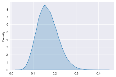
# Generate prior draws
prior_draws = np.random.beta(10, 50, 100000)

# Plot the prior
sns.kdeplot(prior_draws, shade=True, label="prior")
plt.show()

# Extract the banner_clicked column for each product
clothes_clicked = ads.loc[ads["product"] == "clothes"]["banner_clicked"]
sneakers_clicked = ads.loc[ads["product"] == "sneakers"]["banner_clicked"]

# Simulate posterior draws for each product
clothes_posterior = simulate_beta_posterior(clothes_clicked, 10,50)
sneakers_posterior = simulate_beta_posterior(sneakers_clicked, 10,50)
sns.kdeplot(clothes_posterior, shade=True, label="clothes")
sns.kdeplot(sneakers_posterior, shade=True, label="sneakers")
plt.legend(labels=['clothes', 'sneakers'])
plt.show()
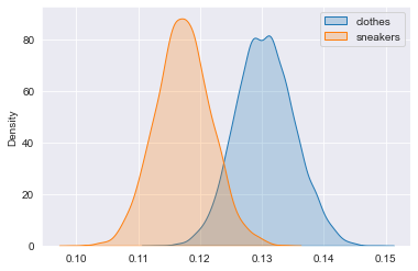
It is more probable that clothes ads are better, but we are not completely sure. We cannot be sure about it, since the two posteriors overlap, so it is actually possible for the sneakers campaign to be bettter.
# Calculate posterior difference and plot it
diff = clothes_posterior - sneakers_posterior
sns.kdeplot(diff, shade=True, label="diff")
plt.axvline(x=0, color='red', linestyle='--')
plt.text(0.0002, 32, "zero difference marker", rotation=90, verticalalignment='center')
plt.title('Difference distribution of clothes - sneakers posteriors')
plt.show()

# Calculate and print 90% credible interval of posterior difference
interval = pm.hdi(diff, hdi_prob=0.9)
print(interval)

# Calculate and print probability of clothes ad being better
clothes_better_prob = (diff > 0).mean()
print(clothes_better_prob)

pm.plot_posterior(np.array(diff), hdi_prob=0.9)
plt.show()
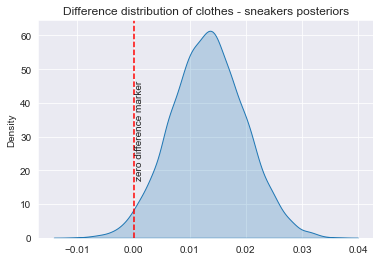
[0.00254178 0.02415007]
0.9795
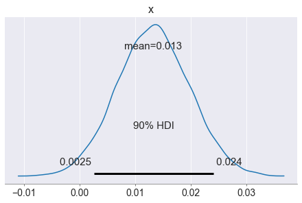
Take a look at the posterior density plot of the difference in click rates: it is very likely positive, indicating that clothes are likely better. The credible interval indicates that with 90% probability, the clothes ads click rate is up to 2.4 percentage points higher than the one for sneakers. Finally, the probability that the clothes click rate is higher is 98%. Great! But there is a 2% chance that actually sneakers ads are better!
Risk analysis
there is a 2% risk that it’s the sneakers ads that are actually better. If that’s the case, how many clicks do we lose if we roll out the clothes campaign?
# Slice diff to take only cases where it is negative
loss = diff[diff < 0]

# Compute and print expected loss
expected_loss = loss.mean()
print(f'maximum loss: {round(expected_loss*100,4)} %')
maximum loss: -0.2422 %
You can safely roll out the clothes campaign to a larger audience. You are 98% sure it has a higher click rare, and even if the 2% risk of this being a wrong decision materializes, you will only lose about 0.2 percentage points in the click rate, which is a very small risk!
Decision analysis
translate parameters to relevant metrics to inform decision making
From posteriors to decisions
- In order to take strategic decisions, one should know the probabilities of different scenarios.
- Bayesian methods allow us to translate parameters into relevant metrics easily.
- Change the unit to which decision takes place in, e.g. CTR dist * impressions * revenue/click = revenue dist
# Calculate distributions of the numbers of clicks for clothes and sneakers
clothes_num_clicks = clothes_posterior * 10_000
sneakers_num_clicks = sneakers_posterior * 10_000

# Calculate cost distributions for each product and platform
ads_costs = {
    "clothes_mobile": clothes_num_clicks * 2.5,
    "sneakers_mobile": sneakers_num_clicks * 2.5,
    "clothes_desktop": clothes_num_clicks * 2,
    "sneakers_desktop": sneakers_num_clicks * 2,
}

# Draw a forest plot of ads_costs
pm.plot_forest(ads_costs, hdi_prob=0.99, textsize=15)
plt.show()
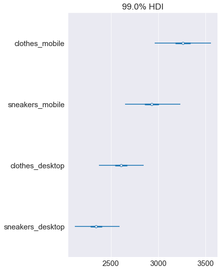
The ends of the whiskers mark the 99% credible interval, so there is a 1% chance the cost will fall outside of it. It’s very, very unlikely, but there is a slim chance that the clothes-mobile cost will turn out lower. It’s important to stay cautious when communicating possible scenarios – that’s the thing with probability, it’s rarely the case that something is ‘completely impossible’!
# Calculate profit distributions for each product and platform
ads_profit = {
    "clothes_mobile": clothes_num_clicks * 3.4 - ads_costs["clothes_mobile"],
    "sneakers_mobile": sneakers_num_clicks * 3.4 - ads_costs["sneakers_mobile"],
    "clothes_desktop": clothes_num_clicks * 3 - ads_costs["clothes_desktop"],
    "sneakers_desktop": sneakers_num_clicks * 3 - ads_costs["sneakers_desktop"],
}

# Draw a forest plot of ads_profit
pm.plot_forest(ads_profit, hdi_prob=0.99)
plt.show()
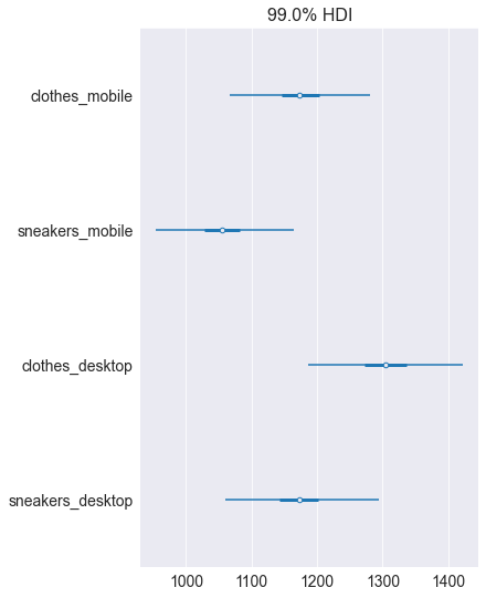
Notice how shifting focus from costs to profit has changed the optimal decision. The sneakers-desktop campaign which minimizes the cost is not the best choice when you care about the profit. Based on these results, you would be more likely to invest in the clothes-desktop campaign, wouldn’t you? Let’s continue to the final lesson of this chapter, where we look at regression and forecasting, the Bayesian way!
Regression and forecasting

Your linear regression model has four parameters: the intercept, the impact of clothes ads, the impact of sneakers ads, and the variance.
Analyzing regression parameters
#list the files
filelist = ['intercept_draws.txt', 'clothes_draws.txt', 'sneakers_draws.txt', 'sd_draws.txt']
#read them into pandas
df_list = [pd.read_csv(file, names=['col']) for file in filelist]
#concatenate them together
posterior_draws_df = pd.concat(df_list, axis=1)
posterior_draws_df.columns=['intercept_draws', 'clothes_draws', 'sneakers_draws', 'sd_draws']

# Describe parameter posteriors
draws_stats = posterior_draws_df.describe()
print(draws_stats)

# Plot clothes parameter posterior
pm.plot_posterior(np.array(posterior_draws_df.clothes_draws), hdi_prob=0.99)
plt.show()
       intercept_draws  clothes_draws  sneakers_draws     sd_draws
count      2000.000000    2000.000000     2000.000000  2000.000000
mean          1.280420       0.104594        0.103594     2.651661
std           0.903845       0.030282        0.031596     0.159491
min          -2.088446      -0.007500        0.001084     2.211899
25%           0.712354       0.085381        0.081577     2.543340
50%           1.288362       0.104680        0.103554     2.639033
75%           1.849244       0.123830        0.125466     2.754714
max           4.343638       0.229886        0.211751     3.278124
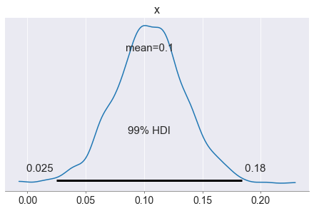
The impact parameters of both clothes and sneakers look okay: they are positive, most likely around 0.1, indicating 1 additional click from 10 ad impressions, which makes sense. Let’s now use the model to make predictions!
Let’s now use the linear regression model to make predictions. How many clicks can we expect if we decide to show 10 clothes ads and 10 sneaker ads?
Predictive distribution
Let’s now use the linear regression model to make predictions. How many clicks can we expect if we decide to show 10 clothes ads and 10 sneaker ads?
# Aggregate posteriors of the parameters to point estimates
intercept_coef = np.mean(posterior_draws_df.intercept_draws)
sneakers_coef = np.mean(posterior_draws_df.sneakers_draws)
clothes_coef = np.mean(posterior_draws_df.clothes_draws)
sd_coef = np.mean(posterior_draws_df.sd_draws)

# Calculate the mean of the predictive distribution
pred_mean = intercept_coef + sneakers_coef * 10 + clothes_coef * 10

# Sample 1000 draws from the predictive distribution
pred_draws = np.random.normal(pred_mean, sd_coef, size=1000)

# Plot the density of the predictive distribution
pm.plot_posterior(pred_draws, hdi_prob=0.99)
plt.show()
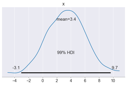
It looks like you can expect more or less three or four clicks if you show 10 clothes and 10 sneaker ads.
Bayesian linear regression with pyMC3
Markov Chain Monte Carlo (MCMC) and model fitting
Problems of Bayesian data analysis in production:
- Grid approximation: inconvenient with many parameters
- Sampling from known posterior: requires conjugate priors
Solution:
- Markov Chains Monte Carlo: sampling from unknown posterior -> same result like others but most flexible
Monte Carlo
Approximating some quantity by generating random numbers
Markov Chains
Markov Chains model a sequence of states, between which one transitions with given probabilities
New Use Case
predict the number of bikes rented per day to plan staff and repairs accordingly
import pandas as pd
import pymc3 as pm
import seaborn as sns
# datacamp has made an error and only provided the test data, no training file downloadable

bikes_test = pd.read_csv('bikes_test.csv')
# very small dataset of just 10 observations
bikes_test.info()
<class 'pandas.core.frame.DataFrame'>
RangeIndex: 10 entries, 0 to 9
Data columns (total 5 columns):
 #   Column      Non-Null Count  Dtype
---  ------      --------------  -----
 0   work_day    10 non-null     int64
 1   temp        10 non-null     float64
 2   humidity    10 non-null     float64
 3   wind_speed  10 non-null     float64
 4   num_bikes   10 non-null     float64
dtypes: float64(4), int64(1)
memory usage: 528.0 bytes
# simple model
formula_first_model = "num_bikes ~ temp + work_day"

# Generate predictive draws
with pm.Model() as model:
    pm.GLM.from_formula(formula_first_model, data=bikes_test,
                       )
    print(model)
    posterior_predictive_first_model = pm.sample(draws=18000, tune=18000, chains=12, cores=6, return_inferencedata=True)
The glm module is deprecated and will be removed in version 4.0
We recommend to instead use Bambi https://bambinos.github.io/bambi/
Auto-assigning NUTS sampler...
Initializing NUTS using jitter+adapt_diag...


Intercept ~ Flat
     temp ~ Normal
 work_day ~ Normal
 sd_log__ ~ TransformedDistribution
       sd ~ HalfCauchy
        y ~ Normal


Multiprocess sampling (12 chains in 6 jobs)
NUTS: [sd, work_day, temp, Intercept]
Sampling 12 chains for 18_000 tune and 18_000 draw iterations (216_000 + 216_000 draws total) took 215 seconds.
There were 1559 divergences after tuning. Increase `target_accept` or reparameterize.
The acceptance probability does not match the target. It is 0.6937498861112372, but should be close to 0.8. Try to increase the number of tuning steps.
There were 1081 divergences after tuning. Increase `target_accept` or reparameterize.
There were 475 divergences after tuning. Increase `target_accept` or reparameterize.
There were 3079 divergences after tuning. Increase `target_accept` or reparameterize.
The acceptance probability does not match the target. It is 0.5765400788999024, but should be close to 0.8. Try to increase the number of tuning steps.
There were 1956 divergences after tuning. Increase `target_accept` or reparameterize.
The acceptance probability does not match the target. It is 0.6623325935424444, but should be close to 0.8. Try to increase the number of tuning steps.
There were 920 divergences after tuning. Increase `target_accept` or reparameterize.
There were 691 divergences after tuning. Increase `target_accept` or reparameterize.
There were 703 divergences after tuning. Increase `target_accept` or reparameterize.
There were 252 divergences after tuning. Increase `target_accept` or reparameterize.
There were 779 divergences after tuning. Increase `target_accept` or reparameterize.
There were 1530 divergences after tuning. Increase `target_accept` or reparameterize.
The acceptance probability does not match the target. It is 0.7154111570610734, but should be close to 0.8. Try to increase the number of tuning steps.
There were 550 divergences after tuning. Increase `target_accept` or reparameterize.
The number of effective samples is smaller than 10% for some parameters.
pm.summary(posterior_predictive_first_model)
| mean | sd | hdi_3% | hdi_97% | mcse_mean | mcse_sd | ess_bulk | ess_tail | r_hat | |
|---|---|---|---|---|---|---|---|---|---|
| Intercept | 0.352 | 0.647 | -0.892 | 1.551 | 0.004 | 0.003 | 29035.0 | 52519.0 | 1.0 |
| temp | 9.050 | 2.919 | 3.644 | 14.619 | 0.017 | 0.012 | 26739.0 | 46236.0 | 1.0 |
| work_day | 0.796 | 0.371 | 0.097 | 1.498 | 0.002 | 0.001 | 34369.0 | 54533.0 | 1.0 |
| sd | 0.396 | 0.147 | 0.190 | 0.651 | 0.002 | 0.001 | 3454.0 | 1887.0 | 1.0 |
# Extend the model with the parameter wind speed

# Define the formula
formula = "num_bikes ~ temp + work_day + wind_speed"

# Generate predictive draws
with pm.Model() as model:
    pm.GLM.from_formula(formula, data=bikes_test,
                       )
    print(model)
    posterior_predictive = pm.sample(draws=18000, tune=18000, chains=12, cores=6, return_inferencedata=True)
The glm module is deprecated and will be removed in version 4.0
We recommend to instead use Bambi https://bambinos.github.io/bambi/


   work_day      temp  humidity  wind_speed  num_bikes
0         0  0.265833  0.687917    0.175996      2.947
1         1  0.282609  0.622174    0.153800      3.784
2         1  0.354167  0.496250    0.147379      4.375
3         1  0.256667  0.722917    0.133721      2.802
4         1  0.265000  0.562083    0.194037      3.830
 Intercept ~ Flat
      temp ~ Normal
  work_day ~ Normal
wind_speed ~ Normal
  sd_log__ ~ TransformedDistribution
        sd ~ HalfCauchy
         y ~ Normal


Auto-assigning NUTS sampler...
Initializing NUTS using jitter+adapt_diag...
Multiprocess sampling (12 chains in 6 jobs)
NUTS: [sd, wind_speed, work_day, temp, Intercept]
Sampling 12 chains for 18_000 tune and 18_000 draw iterations (216_000 + 216_000 draws total) took 322 seconds.
There were 6090 divergences after tuning. Increase `target_accept` or reparameterize.
The acceptance probability does not match the target. It is 0.4535070540886654, but should be close to 0.8. Try to increase the number of tuning steps.
There were 484 divergences after tuning. Increase `target_accept` or reparameterize.
There were 3314 divergences after tuning. Increase `target_accept` or reparameterize.
The acceptance probability does not match the target. It is 0.6322839508323852, but should be close to 0.8. Try to increase the number of tuning steps.
There were 5749 divergences after tuning. Increase `target_accept` or reparameterize.
The acceptance probability does not match the target. It is 0.4657185678254947, but should be close to 0.8. Try to increase the number of tuning steps.
There were 1988 divergences after tuning. Increase `target_accept` or reparameterize.
There were 1572 divergences after tuning. Increase `target_accept` or reparameterize.
There were 3831 divergences after tuning. Increase `target_accept` or reparameterize.
The acceptance probability does not match the target. It is 0.603721265287982, but should be close to 0.8. Try to increase the number of tuning steps.
There were 5848 divergences after tuning. Increase `target_accept` or reparameterize.
The acceptance probability does not match the target. It is 0.4531228873120186, but should be close to 0.8. Try to increase the number of tuning steps.
There were 5826 divergences after tuning. Increase `target_accept` or reparameterize.
The acceptance probability does not match the target. It is 0.47532685097020505, but should be close to 0.8. Try to increase the number of tuning steps.
There were 2830 divergences after tuning. Increase `target_accept` or reparameterize.
The acceptance probability does not match the target. It is 0.6774930920115295, but should be close to 0.8. Try to increase the number of tuning steps.
There were 4966 divergences after tuning. Increase `target_accept` or reparameterize.
The acceptance probability does not match the target. It is 0.528125701676579, but should be close to 0.8. Try to increase the number of tuning steps.
There were 2743 divergences after tuning. Increase `target_accept` or reparameterize.
The acceptance probability does not match the target. It is 0.6825571279708497, but should be close to 0.8. Try to increase the number of tuning steps.
The number of effective samples is smaller than 10% for some parameters.
# 313sec
#pm.save_trace(trace=posterior_predictive, directory='C://Users//SD//Bayes_Theorem_applied_in_Python//trace.dump', overwrite=True)
pm.summary(posterior_predictive)
| mean | sd | hdi_3% | hdi_97% | mcse_mean | mcse_sd | ess_bulk | ess_tail | r_hat | |
|---|---|---|---|---|---|---|---|---|---|
| Intercept | 0.148 | 2.044 | -3.759 | 3.984 | 0.034 | 0.024 | 3097.0 | 5728.0 | 1.01 |
| temp | 9.445 | 4.916 | 0.149 | 18.606 | 0.072 | 0.051 | 3878.0 | 6208.0 | 1.00 |
| work_day | 0.824 | 0.542 | -0.198 | 1.828 | 0.008 | 0.006 | 3356.0 | 10050.0 | 1.01 |
| wind_speed | 0.427 | 4.060 | -7.275 | 8.045 | 0.065 | 0.046 | 3170.0 | 6536.0 | 1.00 |
| sd | 0.471 | 0.190 | 0.224 | 0.793 | 0.006 | 0.004 | 507.0 | 850.0 | 1.03 |
# reference
# https://bookdown.org/rdpeng/advstatcomp/monitoring-convergence.html#gelman-rubin-statistic
# r_hat 1.1 or 1.2 as close to mean that all chains have reasonably converged
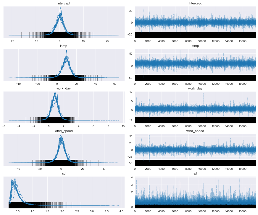
pm.plot_trace(posterior_predictive)
plt.show()
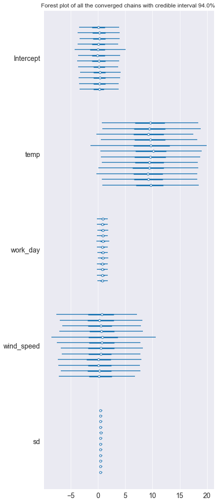
hdi_prob = 0.94
pm.plot_forest(posterior_predictive, hdi_prob=hdi_prob)
plt.title(f'Forest plot of all the converged chains with credible interval {hdi_prob*100}% ')
plt.show()
Interpret results and compare the two models
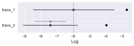
We use the Widely Applicable Information Criterion to compare the two models. Here trace 1 as our first simpler model proves to be better a fit for the data with its higher waic score in pmyc’s comparison function. In the weight column each model’s probability of being the true model is shown, here the extended model with wind speed is clearly worse than the simple one.
import warnings
warnings.simplefilter('ignore')

comparison = pm.compare({"trace_1": posterior_predictive_first_model,
                         "trace_2": posterior_predictive},
                        ic='waic')
comparison
| rank | waic | p_waic | d_waic | weight | se | dse | warning | waic_scale | |
|---|---|---|---|---|---|---|---|---|---|
| trace_1 | 0 | -5.979267 | 3.269994 | 0.000000 | 1.0 | 2.500034 | 0.000000 | True | log |
| trace_2 | 1 | -7.404534 | 3.447594 | 1.425267 | 0.0 | 1.684752 | 0.974662 | True | log |
pm.compareplot(comparison, textsize=13)
# empty circles are the waic scores
# black bars as standard deviations
<AxesSubplot:xlabel='Log'>
Making predictions
# predict with fresh test data
with pm.Model() as model:
    pm.GLM.from_formula(formula_first_model, data=bikes_test)
    predictive_dist = pm.fast_sample_posterior_predictive(posterior_predictive_first_model)
The glm module is deprecated and will be removed in version 4.0
We recommend to instead use Bambi https://bambinos.github.io/bambi/
predictive_dist['y'].shape
(216000, 10)
import numpy as np
import matplotlib.pyplot as plt

# Initialize errors
errors = []

# Iterate over rows of bikes_test to compute error per row
for index, test_example in bikes_test.iterrows():
    error = predictive_dist["y"][:, index] - test_example["num_bikes"]
    errors.append(error)

# Reshape errors
error_distribution = np.array(errors).reshape(-1)

# Plot the error distribution
pm.plot_posterior(error_distribution, kind='hist')
plt.xlim([-3, 3])
plt.show()
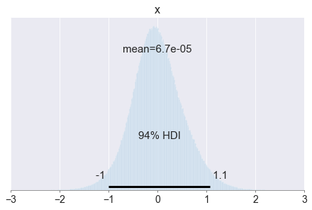
In practice, you might want to compute the error estimate based on more than just 10 observations, but you can already see some patterns. For example, the error is very marginal the error is more often negative than positive, which means that the model tends to underpredict the number of bikes rented!