Non contractual Customer Lifetime Value estimated probabilistically with the Beta Geometric/Negative Binomial Distribution (BG/NBD) Model
We assume an online service business where customers/clients continously purchase our services.
For such a service business we generate our customer transactions ourselves instead of using once again one of the few available public Datasets.
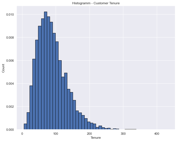
We pick a Gamma distribution for the tenure of our 10000 customers with shape, scale = 4, 11
import numpy as np
import matplotlib.pyplot as plt
import seaborn as sns
sns.set_style('darkgrid')
sns.set(rc={"figure.figsize":(10, 8)})

rng = np.random.default_rng(2022)

shape, scale = 4, 11
tenure = rng.gamma(shape, scale, 10000) *2
plt.hist(tenure, density=True, edgecolor='black', bins=50)
plt.title('Histogramm - Customer Tenure')
plt.xlabel('Tenure')
plt.ylabel('Count')
plt.show()
Using the Beta Geometric/Negative Binomial Distribution (BG/NBD) Model
The BG/NBD is based on the Pareto/NBD model. Unlike to the Pareto/NBD model, the betageometric (BG) model assume that customer die and drop out immideatly after a transaction, whereas Pareto models a probability that dropout with which customers dropout can occurr anytime.
what else is assumed?
-
While active, the number of transactions made by a customer follows a Poisson process with transaction rate $\lambda$, which essentially means the time between transactions is exponentially distributed.
-
Heterogeneity in $ \lambda $ is gamma distributed
-
Customer become inactive with probability p after every transaction inactive with probability $ p $. Therefore the point in time when the customer dies is distributed (shifted) geometrically across transactions
- Heterogeneity in $ p $ follows a beta distribution
-
The transaction rate $ \lambda $ and the dropout probability $ p $ are independent between customers.
Note: $ \lambda $ and $ p $ are both unobserved
All customers are assumed to be active customers in this model, so it makes sense to apply it on a cohort of customers who just have made their first purchase.
let’s generate some daily transactional data for a cohort of fresh customers
%%time
from faker import Faker
import pandas as pd
fake = Faker(['it_IT', 'en_UK', 'fr_FR', 'de_DE', 'uk_UA'])
newcols = fake.simple_profile().keys()

profiles = pd.DataFrame(columns=list(newcols))
for i in range(10000):
    profiles.loc[i] = fake.simple_profile()

profiles['customer_id'] = profiles.index
first_column = profiles.pop('customer_id')
profiles.insert(0, 'customer_id', first_column)
profiles.head()
CPU times: total: 17.2 s
Wall time: 17.3 s
| customer_id | username | name | sex | address | birthdate | ||
|---|---|---|---|---|---|---|---|
| 0 | 0 | abramstey | Nuran Trupp-Lachmann | F | Ritterallee 5/3\n23598 Staffelstein | babett14@hotmail.de | 1952-02-10 |
| 1 | 1 | pichonalex | Marcel Leroy | M | 69, rue de Ollivier\n25378 GoncalvesBourg | francoismartin@club-internet.fr | 1966-12-13 |
| 2 | 2 | le-gallemmanuelle | Monique Roche | F | 85, avenue de Thierry\n67649 Maillet | madeleineleroy@dbmail.com | 1945-04-22 |
| 3 | 3 | jakob73 | Nuray Martin B.Sc. | F | Holtallee 7\n19875 Ahaus | hgeisler@yahoo.de | 1909-09-26 |
| 4 | 4 | shvachkanazar | Тетяна Дергач | F | набережна Лемківська, 2, селище Марʼяна, 101472 | leontii90@email.ua | 1936-08-12 |
# model params rounded from CDNOW sample in the paper p. 281
params=dict()

params['r'] = 0.25,
params['alpha'] = 4.5

params['a'] = 0.8
params['b'] = 2.4

params
{'r': (0.25,), 'alpha': 4.5, 'a': 0.8, 'b': 2.4}
observation_period_end='2021-12-31'
%%time
from lifetimes.generate_data import beta_geometric_nbd_model_transactional_data

transactions = beta_geometric_nbd_model_transactional_data(tenure, params['r'], params['alpha'], params['a'], params['b'],
                                                  observation_period_end=observation_period_end, freq='D', size=10000)
transactions.shape
CPU times: total: 1min 52s
Wall time: 1min 52s


(29664, 2)
trans_df = transactions.merge(profiles, left_on='customer_id', right_on='customer_id')
trans_df.head()
| customer_id | date | username | name | sex | address | birthdate | ||
|---|---|---|---|---|---|---|---|---|
| 0 | 0 | 2021-04-20 21:30:50.384044800 | abramstey | Nuran Trupp-Lachmann | F | Ritterallee 5/3\n23598 Staffelstein | babett14@hotmail.de | 1952-02-10 |
| 1 | 0 | 2021-08-26 06:44:27.043411199 | abramstey | Nuran Trupp-Lachmann | F | Ritterallee 5/3\n23598 Staffelstein | babett14@hotmail.de | 1952-02-10 |
| 2 | 0 | 2021-10-21 23:25:51.052166400 | abramstey | Nuran Trupp-Lachmann | F | Ritterallee 5/3\n23598 Staffelstein | babett14@hotmail.de | 1952-02-10 |
| 3 | 1 | 2021-06-10 07:05:42.827625600 | pichonalex | Marcel Leroy | M | 69, rue de Ollivier\n25378 GoncalvesBourg | francoismartin@club-internet.fr | 1966-12-13 |
| 4 | 1 | 2021-12-11 21:52:01.636838400 | pichonalex | Marcel Leroy | M | 69, rue de Ollivier\n25378 GoncalvesBourg | francoismartin@club-internet.fr | 1966-12-13 |
Aggregate the summary data analog to RFM segmentation (Recency, Frequency, Monetary) from the transactional data just generated
from lifetimes.utils import summary_data_from_transaction_data

summary = summary_data_from_transaction_data(trans_df, 'customer_id', 'date', observation_period_end=observation_period_end)
summary = pd.concat([profiles, summary], axis=1)
summary
| customer_id | username | name | sex | address | birthdate | frequency | recency | T | ||
|---|---|---|---|---|---|---|---|---|---|---|
| 0 | 0 | abramstey | Nuran Trupp-Lachmann | F | Ritterallee 5/3\n23598 Staffelstein | babett14@hotmail.de | 1952-02-10 | 2.0 | 184.0 | 255.0 |
| 1 | 1 | pichonalex | Marcel Leroy | M | 69, rue de Ollivier\n25378 GoncalvesBourg | francoismartin@club-internet.fr | 1966-12-13 | 1.0 | 184.0 | 204.0 |
| 2 | 2 | le-gallemmanuelle | Monique Roche | F | 85, avenue de Thierry\n67649 Maillet | madeleineleroy@dbmail.com | 1945-04-22 | 3.0 | 98.0 | 99.0 |
| 3 | 3 | jakob73 | Nuray Martin B.Sc. | F | Holtallee 7\n19875 Ahaus | hgeisler@yahoo.de | 1909-09-26 | 0.0 | 0.0 | 15.0 |
| 4 | 4 | shvachkanazar | Тетяна Дергач | F | набережна Лемківська, 2, селище Марʼяна, 101472 | leontii90@email.ua | 1936-08-12 | 1.0 | 45.0 | 109.0 |
| ... | ... | ... | ... | ... | ... | ... | ... | ... | ... | ... |
| 9995 | 9995 | iarynahavrylyshyn | Олег Рудько | M | набережна Маркіяна Шашкевича, 517, хутір Данил... | khavrylenko@ukr.net | 1988-07-07 | 0.0 | 0.0 | 40.0 |
| 9996 | 9996 | gisbertriehl | Claire Koch-Anders | F | Zorbachring 7\n70870 Burgdorf | tomas93@hotmail.de | 2014-08-13 | 0.0 | 0.0 | 89.0 |
| 9997 | 9997 | marta63 | Остап Ейбоженко | M | вулиця Бруно Шульца, 915, хутір Ганна, 76375 | vdovychenkobohuslav@meta.ua | 1976-07-24 | 0.0 | 0.0 | 100.0 |
| 9998 | 9998 | opowell | Chelsea Poole | F | Flat 82\nBryan passage\nNorth Luke\nWF1N 0AL | rsmart@hotmail.co.uk | 1916-10-24 | 1.0 | 47.0 | 101.0 |
| 9999 | 9999 | havrylotsymbaliuk | пан Устим Цибуленко | M | вулиця Василя Симоненка, 628, село Леон, 85627 | venedykt92@ukr.net | 1975-02-06 | 2.0 | 44.0 | 75.0 |
10000 rows × 10 columns
"""from lifetimes.generate_data import beta_geometric_nbd_model
#lifetimes.generate_data.beta_geometric_nbd_model(T, r, alpha, a, b, size=1)
#Generate artificial data according to the BG/NBD model.

df = beta_geometric_nbd_model(tenure, params['r'], params['alpha'], params['a'], params['b'], size=10000)
"""
"""Parameters:
T (array_like) – The length of time observing new customers.
alpha, a, b (r,) – Parameters in the model. See [1]_
size (int, optional) – The number of customers to generate
Returns:
DataFrame – With index as customer_ids and the following columns: ‘frequency’, ‘recency’, ‘T’, ‘lambda’, ‘p’, ‘alive’, ‘customer_id’"""
'Parameters:\t\nT (array_like) – The length of time observing new customers.\nalpha, a, b (r,) – Parameters in the model. See [1]_\nsize (int, optional) – The number of customers to generate\nReturns:\t\nDataFrame – With index as customer_ids and the following columns: ‘frequency’, ‘recency’, ‘T’, ‘lambda’, ‘p’, ‘alive’, ‘customer_id’'
from lifetimes import BetaGeoFitter
bgf = BetaGeoFitter(penalizer_coef=0)
bgf.fit(summary['frequency'], summary['recency'], summary['T'])
bgf.summary
| coef | se(coef) | lower 95% bound | upper 95% bound | |
|---|---|---|---|---|
| r | 0.289300 | 0.005818 | 0.277897 | 0.300704 |
| alpha | 6.476316 | 0.213714 | 6.057437 | 6.895194 |
| a | 0.790777 | 0.053952 | 0.685031 | 0.896524 |
| b | 2.530743 | 0.231390 | 2.077220 | 2.984267 |
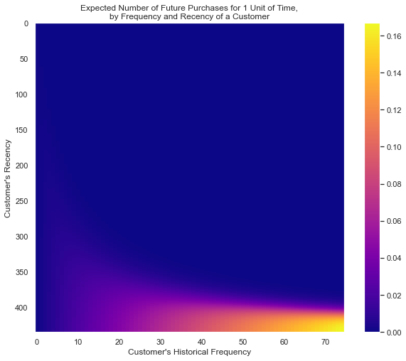
from lifetimes.plotting import plot_frequency_recency_matrix
sns.set(rc={"figure.figsize":(10, 8)})
sns.set_style('dark')
plot_frequency_recency_matrix(bgf, cmap='plasma')
plt.show()
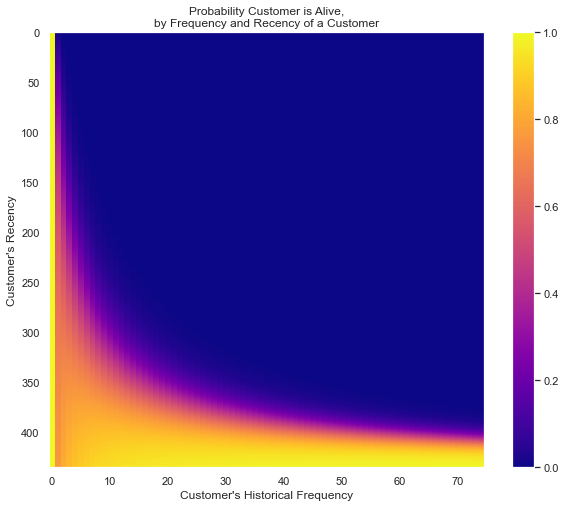
from lifetimes.plotting import plot_probability_alive_matrix

plot_probability_alive_matrix(bgf, cmap='plasma')
plt.show()
Customer ranking
Let us identify the customers with Top 5 expected purchases within next seven days (t=7) based on their transaction history.
t = 7
ppcolname = 'predicted_purchases_' + str(t)
summary[ppcolname] = bgf.conditional_expected_number_of_purchases_up_to_time(t, summary['frequency'],summary['recency'], summary['T'])
summary.sort_values(by=ppcolname, ascending=False).head(5)
| customer_id | username | name | sex | address | birthdate | frequency | recency | T | predicted_purchases_14 | predicted_purchases_30 | predicted_purchases_7 | monetary_value_average | Expected_cond_average_revenue | error_rev | ||
|---|---|---|---|---|---|---|---|---|---|---|---|---|---|---|---|---|
| 2910 | 2910 | carlypalmer | Mrs. Joan Heath | M | Studio 41t\nAbigail port\nEast Jayne\nPO5X 1DL | sally36@yahoo.co.uk | 1908-01-15 | 33.0 | 55.0 | 55.0 | 6.851758 | 14.839702 | 3.557546 | 38.734677 | 38.622364 | -0.112313 |
| 3129 | 3129 | jsontag | Zeynep Steckel | F | Biengasse 720\n46808 Ansbach | peukertmeike@aol.de | 1976-05-28 | 20.0 | 30.0 | 31.0 | 6.324447 | 13.947335 | 3.344909 | 31.671466 | 31.566594 | -0.104872 |
| 1677 | 1677 | bohodarokhrimenko | Болеслав Дубас | M | вулиця Шота Руставелі, 248, місто Лариса, 11399 | artemtymchuk@gmail.com | 1974-01-16 | 19.0 | 34.0 | 34.0 | 5.749406 | 12.524436 | 3.029490 | 16.370829 | 16.441952 | 0.071123 |
| 3149 | 3149 | ujones | Kieran Jennings | F | Flat 3\nRoger port\nKieranton\nSR3 0HP | abigailphillips@gmail.com | 2012-02-22 | 34.0 | 71.0 | 72.0 | 5.554099 | 12.087839 | 2.862532 | 7.135654 | 7.237132 | 0.101478 |
| 7500 | 7500 | elombardi | Dott. Melania Toldo | F | Incrocio Bragaglia 3\nCostanzi sardo, 94137 Tr... | cgagliano@tim.it | 2016-02-24 | 23.0 | 47.0 | 47.0 | 5.412396 | 11.756576 | 2.821701 | 12.182490 | 12.282481 | 0.099991 |
t = 30
ppcolname = 'predicted_purchases_' + str(t)
summary[ppcolname] = bgf.conditional_expected_number_of_purchases_up_to_time(t, summary['frequency'],summary['recency'], summary['T'])
sorted_summary = summary.sort_values(by=ppcolname, ascending=False)
sorted_summary.head()
| customer_id | username | name | sex | address | birthdate | frequency | recency | T | predicted_purchases_14 | predicted_purchases_30 | predicted_purchases_7 | monetary_value_average | Expected_cond_average_revenue | error_rev | ||
|---|---|---|---|---|---|---|---|---|---|---|---|---|---|---|---|---|
| 2910 | 2910 | carlypalmer | Mrs. Joan Heath | M | Studio 41t\nAbigail port\nEast Jayne\nPO5X 1DL | sally36@yahoo.co.uk | 1908-01-15 | 33.0 | 55.0 | 55.0 | 6.851758 | 13.594318 | 3.557546 | 38.734677 | 38.622364 | -0.112313 |
| 3129 | 3129 | jsontag | Zeynep Steckel | F | Biengasse 720\n46808 Ansbach | peukertmeike@aol.de | 1976-05-28 | 20.0 | 30.0 | 31.0 | 6.324447 | 12.149527 | 3.344909 | 31.671466 | 31.566594 | -0.104872 |
| 3149 | 3149 | ujones | Kieran Jennings | F | Flat 3\nRoger port\nKieranton\nSR3 0HP | abigailphillips@gmail.com | 2012-02-22 | 34.0 | 71.0 | 72.0 | 5.554099 | 11.173048 | 2.862532 | 7.135654 | 7.237132 | 0.101478 |
| 1677 | 1677 | bohodarokhrimenko | Болеслав Дубас | M | вулиця Шота Руставелі, 248, місто Лариса, 11399 | artemtymchuk@gmail.com | 1974-01-16 | 19.0 | 34.0 | 34.0 | 5.749406 | 11.114488 | 3.029490 | 16.370829 | 16.441952 | 0.071123 |
| 7500 | 7500 | elombardi | Dott. Melania Toldo | F | Incrocio Bragaglia 3\nCostanzi sardo, 94137 Tr... | cgagliano@tim.it | 2016-02-24 | 23.0 | 47.0 | 47.0 | 5.412396 | 10.659459 | 2.821701 | 12.182490 | 12.282481 | 0.099991 |
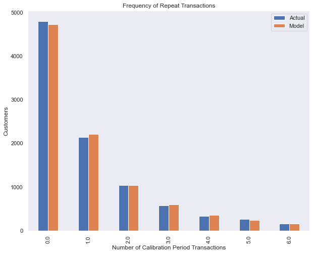
Model fit assessment
from lifetimes.plotting import plot_period_transactions
plot_period_transactions(bgf)
plt.show()
calibration_period_end='2021-10-10'
from lifetimes.utils import calibration_and_holdout_data

summary_cal_holdout = calibration_and_holdout_data(trans_df, 'customer_id', 'date',
                                        calibration_period_end=calibration_period_end,
                                        observation_period_end=observation_period_end )
summary_cal_holdout.info()
<class 'pandas.core.frame.DataFrame'>
Int64Index: 4998 entries, 0 to 9998
Data columns (total 5 columns):
 #   Column             Non-Null Count  Dtype
---  ------             --------------  -----
 0   frequency_cal      4998 non-null   float64
 1   recency_cal        4998 non-null   float64
 2   T_cal              4998 non-null   float64
 3   frequency_holdout  4998 non-null   float64
 4   duration_holdout   4998 non-null   float64
dtypes: float64(5)
memory usage: 363.3 KB
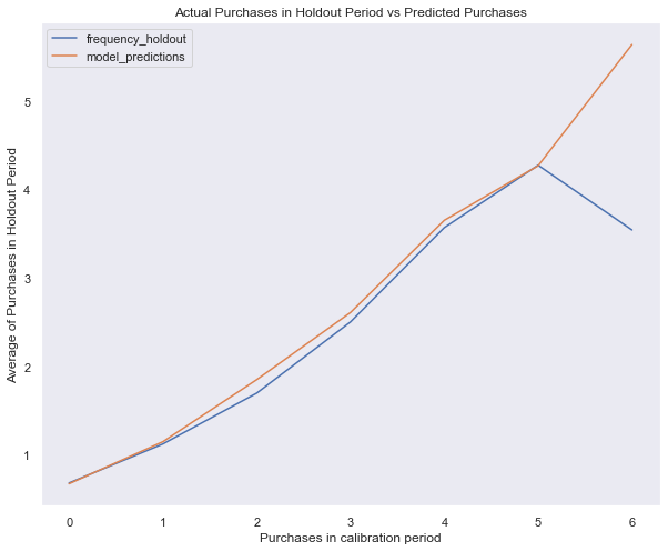
from lifetimes.plotting import plot_calibration_purchases_vs_holdout_purchases

bgf = BetaGeoFitter(penalizer_coef=0.001)
bgf.fit(summary_cal_holdout['frequency_cal'], summary_cal_holdout['recency_cal'], summary_cal_holdout['T_cal'])
plot_calibration_purchases_vs_holdout_purchases(bgf, summary_cal_holdout)
plt.show()
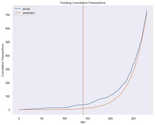
bgf.fit(summary_cal_holdout['frequency_cal'], summary_cal_holdout['recency_cal'], summary_cal_holdout['T_cal'])
plot_cumulative_transactions(bgf, trans_df, 'date', 'customer_id', 280, 140);
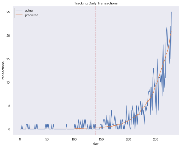
plot_incremental_transactions(bgf, trans_df, 'date', 'customer_id',280, 140);
customer_X = sorted_summary[200:201]
customer_X
| customer_id | username | name | sex | address | birthdate | frequency | recency | T | predicted_purchases_14 | predicted_purchases_30 | predicted_purchases_7 | monetary_value_average | Expected_cond_average_revenue | error_rev | ||
|---|---|---|---|---|---|---|---|---|---|---|---|---|---|---|---|---|
| 8403 | 8403 | trubinguenther | Ing. Hanno Ullmann | M | Gudegasse 8/4\n87671 Grevenbroich | riehlmarlen@yahoo.de | 1909-03-31 | 7.0 | 44.0 | 46.0 | 1.601542 | 3.179439 | 0.831359 | 18.652597 | 18.769815 | 0.117218 |
t = 30 # predict number of purchases in next t periods

individual = summary.iloc[customer_X.customer_id]
bgf.predict(t, individual['frequency'], individual['recency'], individual['T'])
# 0.0576511
8403    3.374978
dtype: float64
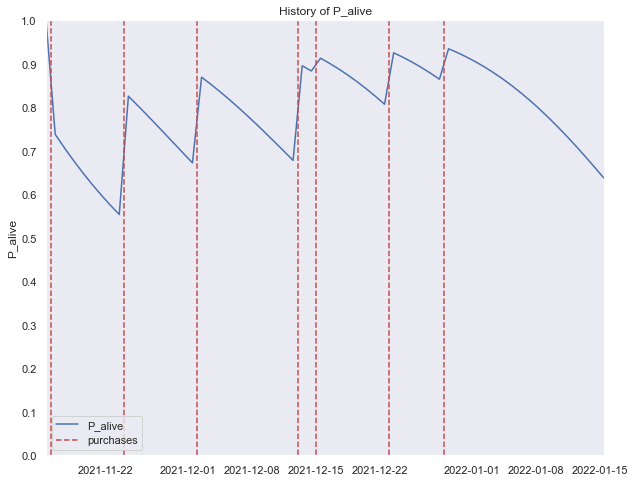
from lifetimes.plotting import plot_history_alive

days_since_birth = 61 # of this customer X

sp_trans = trans_df.loc[trans_df['customer_id'] == int(customer_X.customer_id)]
plot_history_alive(bgf, days_since_birth, sp_trans, 'date', title='History of P_alive of customer_X='+str(customer_X.username) )
plt.show()
sp_trans
| customer_id | date | username | name | sex | address | birthdate | ||
|---|---|---|---|---|---|---|---|---|
| 25086 | 8403 | 2021-11-15 11:51:07.696598400 | trubinguenther | Ing. Hanno Ullmann | M | Gudegasse 8/4\n87671 Grevenbroich | riehlmarlen@yahoo.de | 1909-03-31 |
| 25087 | 8403 | 2021-11-16 21:17:22.970515200 | trubinguenther | Ing. Hanno Ullmann | M | Gudegasse 8/4\n87671 Grevenbroich | riehlmarlen@yahoo.de | 1909-03-31 |
| 25088 | 8403 | 2021-11-24 04:46:07.064832 | trubinguenther | Ing. Hanno Ullmann | M | Gudegasse 8/4\n87671 Grevenbroich | riehlmarlen@yahoo.de | 1909-03-31 |
| 25089 | 8403 | 2021-12-02 19:17:03.481641600 | trubinguenther | Ing. Hanno Ullmann | M | Gudegasse 8/4\n87671 Grevenbroich | riehlmarlen@yahoo.de | 1909-03-31 |
| 25090 | 8403 | 2021-12-13 04:24:15.312902400 | trubinguenther | Ing. Hanno Ullmann | M | Gudegasse 8/4\n87671 Grevenbroich | riehlmarlen@yahoo.de | 1909-03-31 |
| 25091 | 8403 | 2021-12-15 16:12:24.811142400 | trubinguenther | Ing. Hanno Ullmann | M | Gudegasse 8/4\n87671 Grevenbroich | riehlmarlen@yahoo.de | 1909-03-31 |
| 25092 | 8403 | 2021-12-23 23:41:56.826096 | trubinguenther | Ing. Hanno Ullmann | M | Gudegasse 8/4\n87671 Grevenbroich | riehlmarlen@yahoo.de | 1909-03-31 |
| 25093 | 8403 | 2021-12-29 12:19:29.010403200 | trubinguenther | Ing. Hanno Ullmann | M | Gudegasse 8/4\n87671 Grevenbroich | riehlmarlen@yahoo.de | 1909-03-31 |
no_transactions = trans_df.groupby('customer_id').count().sort_values('date', ascending=False)['date']
no_transactions
customer_id
2019    88
5280    87
985     75
7987    66
7892    57
        ..
1722     1
5653     1
5651     1
5650     1
6404     1
Name: date, Length: 10000, dtype: int64
df3 = summary[summary['frequency']>0]
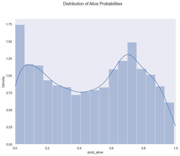
df3['prob_alive'] = bgf.conditional_probability_alive(df3['frequency'],df3['recency'],df3['T'])
sns.distplot(df3['prob_alive']);
plt.xlim(0,1)
plt.suptitle('Distribution of Alive Probabilities')
plt.show()
df3['churn'] = ['churned' if p < .1 else 'not churned' for p in df3['prob_alive']]
sns.countplot(df3['churn']);
plt.suptitle('Grouping of alive probabilities')
plt.show()
print('Grouping of alive probabilities')
df3['churn'][(df3['prob_alive']>=.1) & (df3['prob_alive']<.2)] = "high risk"
df3['churn'].value_counts()
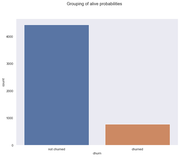
Grouping of alive probabilities


not churned    3841
churned         772
high risk       589
Name: churn, dtype: int64
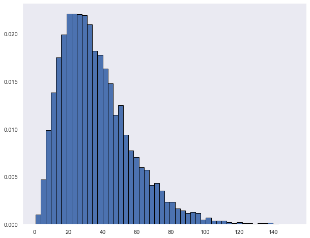
Model monetary transaction value data modeled with Gamma-Gamma model
## monetray value data gen

shape, scale = 3, 3.  # mean=4, std=2*sqrt(2)
monetary_value_average = rng.gamma(shape, scale, 10000) * 2
plt.hist(monetary_value_average*2, density=True, edgecolor='black', bins=50)
plt.show()
summary['monetary_value_average'] = transaction_amount

returning_customers_summary = summary[summary['frequency']>0]
returning_customers_summary.head()
| customer_id | username | name | sex | address | birthdate | frequency | recency | T | predicted_purchases_14 | predicted_purchases_30 | predicted_purchases_7 | monetary_value_average | Expected_cond_average_revenue | error_rev | ||
|---|---|---|---|---|---|---|---|---|---|---|---|---|---|---|---|---|
| 0 | 0 | abramstey | Nuran Trupp-Lachmann | F | Ritterallee 5/3\n23598 Staffelstein | babett14@hotmail.de | 1952-02-10 | 2.0 | 184.0 | 255.0 | 0.082734 | 0.174773 | 0.041632 | 32.613560 | 31.565017 | -1.048543 |
| 1 | 1 | pichonalex | Marcel Leroy | M | 69, rue de Ollivier\n25378 GoncalvesBourg | francoismartin@club-internet.fr | 1966-12-13 | 1.0 | 184.0 | 204.0 | 0.062412 | 0.131735 | 0.031418 | 16.727437 | 17.774840 | 1.047403 |
| 2 | 2 | le-gallemmanuelle | Monique Roche | F | 85, avenue de Thierry\n67649 Maillet | madeleineleroy@dbmail.com | 1945-04-22 | 3.0 | 98.0 | 99.0 | 0.357496 | 0.738755 | 0.181780 | 8.692225 | 9.658282 | 0.966057 |
| 4 | 4 | shvachkanazar | Тетяна Дергач | F | набережна Лемківська, 2, селище Марʼяна, 101472 | leontii90@email.ua | 1936-08-12 | 1.0 | 45.0 | 109.0 | 0.080884 | 0.168804 | 0.040935 | 14.807318 | 16.211255 | 1.403937 |
| 5 | 5 | petro07 | Алла Рябець | F | набережна Дністровська, 843, хутір Ілля, 106205 | sviatoslavadurdynets@ukr.net | 2002-08-12 | 1.0 | 6.0 | 34.0 | 0.172044 | 0.345416 | 0.088817 | 25.410872 | 24.845904 | -0.564968 |
Important assumption for the Gamma-Gamma Model: the relationship between the monetary value and the purchase frequency is near zero.
As this is met we can continue to train the model and start analysing.
returning_customers_summary[['monetary_value_average', 'frequency']].corr()
| monetary_value_average | frequency | |
|---|---|---|
| monetary_value_average | 1.00000 | -0.00149 |
| frequency | -0.00149 | 1.00000 |
from lifetimes import GammaGammaFitter

ggf = GammaGammaFitter(penalizer_coef = 0.002)
ggf.fit(returning_customers_summary['frequency'], returning_customers_summary['monetary_value_average'])
<lifetimes.GammaGammaFitter: fitted with 5202 subjects, p: 5.53, q: 2.26, v: 5.10>
ggf.summary
| coef | se(coef) | lower 95% bound | upper 95% bound | |
|---|---|---|---|---|
| p | 5.532698 | 0.115701 | 5.305924 | 5.759472 |
| q | 2.261587 | 0.044056 | 2.175237 | 2.347938 |
| v | 5.100490 | 0.125329 | 4.854845 | 5.346135 |
summary['Expected_cond_average_revenue'] = ggf.conditional_expected_average_profit(summary['frequency'], summary['monetary_value_average'])
summary['Expected_cond_average_revenue'].describe()
count    10000.000000
mean        20.413614
std          7.062209
min          1.499528
25%         16.409391
50%         22.368232
75%         22.368232
max         75.235044
Name: Expected_cond_average_revenue, dtype: float64
# MAPE
from sklearn.metrics import mean_absolute_percentage_error

summary["error_rev"] = summary['Expected_cond_average_revenue'] - summary['monetary_value_average']

mape = mean_absolute_percentage_error(summary['Expected_cond_average_revenue'], summary["monetary_value_average"])
print("MAPE of predicted revenues:", f'{mape:.3f}')
MAPE of predicted revenues: 0.244
summary['Expected_cond_average_revenue'].head(20)
0     31.565017
1     17.774840
2      9.658282
3     22.368232
4     16.211255
5     24.845904
6     22.368232
7     22.368232
8     22.368232
9      8.200775
10    23.078353
11     6.811015
12     9.628732
13    22.368232
14    22.368232
15    22.368232
16    19.063189
17    29.568306
18    34.173798
19    12.974695
Name: Expected_cond_average_revenue, dtype: float64
print("Expected conditional average profit: %s vs. Average profit: %s" % (
    ggf.conditional_expected_average_profit(
        summary['frequency'],
        summary['monetary_value_average']
    ).mean(),
    summary[summary['frequency']>0]['monetary_value_average'].mean()
))
Expected conditional average profit: 20.41361394230678 vs. Average profit: 18.131239279823276
Calculate the Customer Lifetime Value disconted by DCF and a annual interest rate
# refit the BG model
bgf.fit(summary['frequency'], summary['recency'], summary['T'])

# modelling CLV
summary['clv'] = ggf.customer_lifetime_value(
    bgf,
    summary['frequency'],
    summary['recency'],
    summary['T'],
    summary['monetary_value_average'],
    time=12, # lifetime in months
    discount_rate=0.006
)
summary['clv'].head(10)
0   52.30111846
1   20.98403156
2   57.38228431
3   47.29754080
4   21.46389456
5   52.60841130
6   14.31632335
7   27.28834943
8   14.72406602
9   15.56113740
Name: clv, dtype: float64
# describe the distribution
pd.options.display.float_format = '{:.8f}'.format
summary['clv'].describe()
count   10000.00000000
mean       56.73016752
std       142.07256046
min         0.00000003
25%        13.83895220
50%        21.00412658
75%        39.37786598
max      3623.81967049
Name: clv, dtype: float64
ax = sns.distplot(summary['clv'], kde=False, rug=True)
ax.set_yscale('log')
plt.suptitle('Distribution of Customer Lifetime Value vs. logarithmic density')

plt.show()
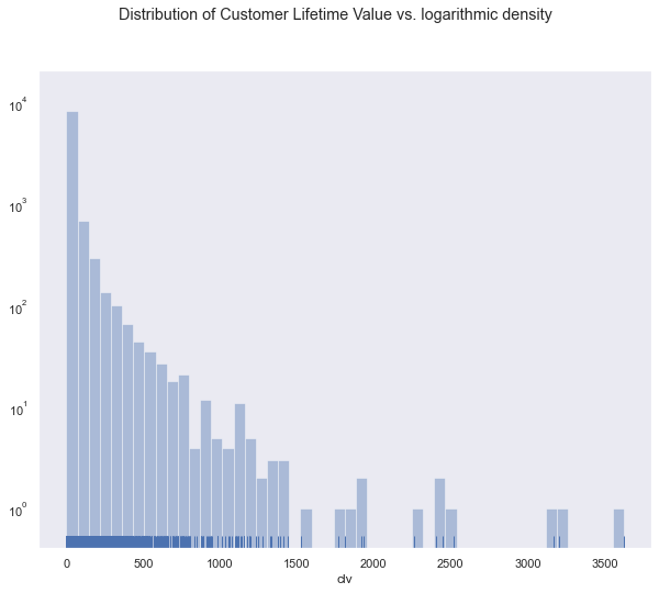
Although the 75% percentile is at under 40 bucks, few customers with high variance and 4 digit CLV lift the arithmetic mean of CLV way above that number.
It makes sense to segment these different customer types differently to better approach them. The features from this BG/NBD have been engineered and can be used for such a customer segmentation.
Compare with the original summary df and look at all these new columns:
summary.columns
Index(['customer_id', 'username', 'name', 'sex', 'address', 'mail',
       'birthdate', 'frequency', 'recency', 'T', 'predicted_purchases_14',
       'predicted_purchases_30', 'predicted_purchases_7',
       'monetary_value_average', 'Expected_cond_average_revenue', 'error_rev',
       'clv'],
      dtype='object')
References