Are You Ready for the Zombie Apocalypse - Datacamp R project in Statsmodels (Python)
Concept and R Version: datacamp
1. ZOMBIES!
News reports suggest that the impossible has become possible…zombies have appeared on the streets of the US! What should we do? The Centers for Disease Control and Prevention (CDC) zombie preparedness website recommends storing water, food, medication, tools, sanitation items, clothing, essential documents, and first aid supplies. Thankfully, we are CDC analysts and are prepared, but it may be too late for others!
Our team decides to identify supplies that protect people and coordinate supply distribution. A few brave data collectors volunteer to check on 200 randomly selected adults who were alive before the zombies. We have recent data for the 200 on age and sex, how many are in their household, and their rural, suburban, or urban location. Our heroic volunteers visit each home and record zombie status and preparedness. Now it's our job to figure out which supplies are associated with safety!

import pandas as pd

# Read in the data
zombies = pd.read_csv("datasets/zombies.csv")

# Examine the data with summary()
print(zombies.info())

# Create water-per-person
zombies['water_per_person'] = zombies.water / zombies.household

# Examine the new variable
print('\n\n' + str(zombies['water_per_person'].describe()))

zombies.head(2)
<class 'pandas.core.frame.DataFrame'>
RangeIndex: 200 entries, 0 to 199
Data columns (total 14 columns):
 #   Column      Non-Null Count  Dtype
---  ------      --------------  -----
 0   zombieid    200 non-null    int64
 1   zombie      200 non-null    object
 2   age         200 non-null    int64
 3   sex         200 non-null    object
 4   rurality    200 non-null    object
 5   household   200 non-null    int64
 6   water       200 non-null    int64
 7   food        200 non-null    object
 8   medication  200 non-null    object
 9   tools       200 non-null    object
 10  firstaid    200 non-null    object
 11  sanitation  200 non-null    object
 12  clothing    126 non-null    object
 13  documents   66 non-null     object
dtypes: int64(4), object(10)
memory usage: 22.0+ KB
None


count    200.000000
mean       3.091833
std        3.627677
min        0.000000
25%        0.000000
50%        2.000000
75%        5.333333
max       13.333333
Name: water_per_person, dtype: float64
| zombieid | zombie | age | sex | rurality | household | water | food | medication | tools | firstaid | sanitation | clothing | documents | water_per_person | |
|---|---|---|---|---|---|---|---|---|---|---|---|---|---|---|---|
| 0 | 1 | Human | 18 | Female | Rural | 1 | 0 | Food | Medication | No tools | First aid supplies | Sanitation | Clothing | NaN | 0.0 |
| 1 | 2 | Human | 18 | Male | Rural | 3 | 24 | Food | Medication | tools | First aid supplies | Sanitation | Clothing | NaN | 8.0 |
2. Compare zombies and humans
Because every moment counts when dealing with life and (un)death, we want to get this right! The first task is to compare humans and zombies to identify differences in supplies. We review the data and find the following:
- zombieid: unique identifier
- zombie: human or zombie
- age: age in years
- sex: male or female
- rurality: rural, suburban, or urban
- household: number of people living in household
- water: gallons of clean water available
- food: food or no food
- medication: medication or no medication
- tools: tools or no tools
- firstaid: first aid or no first aid
- sanitation: sanitation or no sanitation
- clothing: clothing or no clothing
- documents: documents or no documents
# import matplotlib and seaborn
import matplotlib.pyplot as plt
import seaborn as sns
sns.set_style('darkgrid')
# Display plots side by side
plt.figure(figsize=(12,6))
plt.subplot(1,2,1)
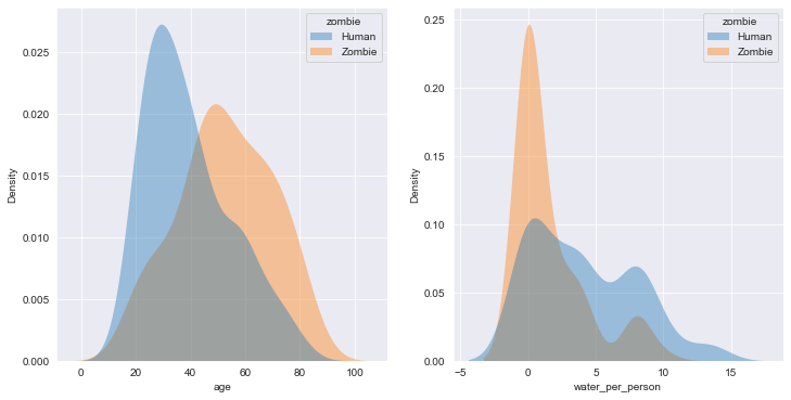
sns.kdeplot(data=zombies, x='age', hue="zombie",
#multiple="fill" ,
fill=True,
alpha=.4, linewidth=0,
common_norm=False,
legend=True)
plt.subplot(1,2,2)
sns.kdeplot(data=zombies, x='water_per_person', hue="zombie",
#multiple="fill" ,
fill=True,
alpha=.4, linewidth=0,
common_norm=False,
legend=True)
plt.show()
3. Compare zombies and humans (part 2)
It looks like those who turned into zombies were older and had less available clean water. This suggests that getting water to the remaining humans might help protect them from the zombie hoards! Protecting older citizens is important, so we need to think about the best ways to reach this group. What are the other characteristics and supplies that differ between humans and zombies? Do zombies live in urban areas? Or are they more common in rural areas? Is water critical to staying human? Is food critical to staying human?

Let us determine the percentage of zombies for each category of the factor variables.
# calc zombie sample proportions
import numpy as np
zombies.select_dtypes(include=np.number)

zombies_categoricals = zombies.loc[:,zombies.select_dtypes(exclude=np.number).columns]

for column in zombies_categoricals.columns:
    freq = pd.crosstab(zombies[column], zombies.zombie, margins=True)
    print(freq.div(freq["All"],axis=0))
    print('\n')
zombie  Human  Zombie  All
zombie
Human   1.000   0.000  1.0
Zombie  0.000   1.000  1.0
All     0.605   0.395  1.0


zombie     Human    Zombie  All
sex
Female  0.626263  0.373737  1.0
Male    0.584158  0.415842  1.0
All     0.605000  0.395000  1.0


zombie       Human    Zombie  All
rurality
Rural     0.816327  0.183673  1.0
Suburban  0.520833  0.479167  1.0
Urban     0.296296  0.703704  1.0
All       0.605000  0.395000  1.0


zombie      Human    Zombie  All
food
Food     0.827273  0.172727  1.0
No food  0.333333  0.666667  1.0
All      0.605000  0.395000  1.0


zombie            Human    Zombie  All
medication
Medication     0.829787  0.170213  1.0
No medication  0.405660  0.594340  1.0
All            0.605000  0.395000  1.0


zombie       Human    Zombie  All
tools
No tools  0.603960  0.396040  1.0
tools     0.606061  0.393939  1.0
All       0.605000  0.395000  1.0


zombie                    Human    Zombie  All
firstaid
First aid supplies     0.632075  0.367925  1.0
No first aid supplies  0.574468  0.425532  1.0
All                    0.605000  0.395000  1.0


zombie            Human    Zombie  All
sanitation
No sanitation  0.470588  0.529412  1.0
Sanitation     0.744898  0.255102  1.0
All            0.605000  0.395000  1.0


zombie       Human    Zombie  All
clothing
Clothing  0.587302  0.412698  1.0
All       0.587302  0.412698  1.0


zombie        Human    Zombie  All
documents
Documents  0.666667  0.333333  1.0
All        0.666667  0.333333  1.0
4. Recode variables missing values
Hmm…it seems a little fishy that the clothing and documents variables have only one category in prop.table(). After checking with the data collectors, they told you that they recorded those without clothing or documents as missing values or NA rather than No clothing or No documents.
To make sure the analyses are consistent and useful, the analysis team leader decides we should recode the NA values to No clothing and No documents for these two variables.
zombies.clothing.fillna('None',inplace=True)
zombies.documents.fillna('None',inplace=True)

# Check recoding
zombies.info() # now both cols have 200 records
zombies[['clothing', 'documents']].sample(3)
<class 'pandas.core.frame.DataFrame'>
RangeIndex: 200 entries, 0 to 199
Data columns (total 15 columns):
 #   Column            Non-Null Count  Dtype
---  ------            --------------  -----
 0   zombieid          200 non-null    int64
 1   zombie            200 non-null    object
 2   age               200 non-null    int64
 3   sex               200 non-null    object
 4   rurality          200 non-null    object
 5   household         200 non-null    int64
 6   water             200 non-null    int64
 7   food              200 non-null    object
 8   medication        200 non-null    object
 9   tools             200 non-null    object
 10  firstaid          200 non-null    object
 11  sanitation        200 non-null    object
 12  clothing          200 non-null    object
 13  documents         200 non-null    object
 14  water_per_person  200 non-null    float64
dtypes: float64(1), int64(4), object(10)
memory usage: 23.6+ KB
| clothing | documents | |
|---|---|---|
| 164 | Clothing | None |
| 51 | None | None |
| 87 | None | None |
5. Selecting variables to predict zombie status
From Task 3, it appears that 70.4% of people in urban areas are zombies, while just 18.4% of those in rural areas are zombies. Getting humans out of cities and protecting those who cannot leave seems important!
For most of the supplies, there is less of a difference between humans and zombies, so it is difficult to decide what else to do. Since there is just one chance to get it right and every minute counts, the analysis team decides to conduct bivariate statistical tests to gain a better understanding of which differences in percents are statistically significantly associated with being a human or a zombie.
# Update subset of factors
zombies_categoricals = zombies.loc[:,zombies.select_dtypes(exclude=np.number).columns]

# Pearson's Chi-squared for categorical features
# H0: no relation between the variables
from scipy.stats import chi2_contingency
testrecords = pd.DataFrame(columns=['stat', 'p', 'dof', 'expected']).T

for column in zombies_categoricals.columns:
    freq = pd.crosstab(zombies[column], zombies.zombie)
    testrecords[column] = chi2_contingency(freq)

# Two sample t-tests for numerical features
from scipy.stats import ttest_ind
#from statsmodels.stats.weightstats import ttest_ind

#perform two sample t-test
zombies['zombie'] = zombies['zombie'].map({'Zombie':1, 'Human':0})

ttestage= ttest_ind(zombies.age, zombies['zombie'], equal_var = False)
ttestwater = ttest_ind(zombies.water, zombies['zombie'], equal_var = False)
print(ttestage, '\n', ttestwater)

testrecords.T
Ttest_indResult(statistic=35.821671560453694, pvalue=8.609943386215585e-89)
 Ttest_indResult(statistic=9.78160028588796, pvalue=1.041125186652482e-18)
| stat | p | dof | expected | |
|---|---|---|---|---|
| zombie | 195.83735 | 0.0 | 1 | [[73.205, 47.795], [47.795, 31.205]] |
| sex | 0.215611 | 0.642405 | 1 | [[59.895, 39.105], [61.105, 39.895]] |
| rurality | 41.27083 | 0.0 | 2 | [[59.29, 38.71], [29.04, 18.96], [32.67, 21.33]] |
| food | 48.490132 | 0.0 | 1 | [[66.55, 43.45], [54.45, 35.55]] |
| medication | 35.747219 | 0.0 | 1 | [[56.87, 37.13], [64.13, 41.87]] |
| tools | 0.0 | 1.0 | 1 | [[61.105, 39.895], [59.895, 39.105]] |
| firstaid | 0.471781 | 0.492169 | 1 | [[64.13, 41.87], [56.87, 37.13]] |
| sanitation | 14.610225 | 0.000132 | 1 | [[61.71, 40.29], [59.29, 38.71]] |
| clothing | 0.268638 | 0.604247 | 1 | [[76.23, 49.77], [44.77, 29.23]] |
| documents | 1.20605 | 0.272116 | 1 | [[39.93, 26.07], [81.07, 52.93]] |
Apart from zombies which cannot be independent of themselves are these features: rurality, food, medication and sanitation.
6. Build the model
Now we are getting somewhere! Rurality, food, medication, sanitation, age, and water per person have statistically significant relationships to zombie status. We use this information to coordinate the delivery of food and medication while we continue to examine the data!
The next step is to estimate a logistic regression model with zombie as the outcome. The generalized linear model command, glm(), can be used to determine whether and how each variable, and the set of variables together, contribute to predicting zombie status. Following glm(), odds.n.ends() computes model significance, fit, and odds ratios.
import statsmodels.api as sm
import statsmodels.formula.api as smf

formula = "zombie ~ age + water_per_person + C(food) + C(rurality) + C(medication) + C(sanitation)"
model = sm.GLM.from_formula(formula=formula, data=zombies, family=sm.families.Binomial()).fit()
print(model.summary())
                 Generalized Linear Model Regression Results
==============================================================================
Dep. Variable:                 zombie   No. Observations:                  200
Model:                            GLM   Df Residuals:                      192
Model Family:                Binomial   Df Model:                            7
Link Function:                  logit   Scale:                          1.0000
Method:                          IRLS   Log-Likelihood:                -61.388
Date:                Tue, 23 Nov 2021   Deviance:                       122.78
Time:                        11:54:59   Pearson chi2:                     440.
No. Iterations:                     7   Pseudo R-squ. (CS):             0.5171
Covariance Type:            nonrobust
==================================================================================================
                                     coef    std err          z      P>|z|      [0.025      0.975]
--------------------------------------------------------------------------------------------------
Intercept                         -6.0986      1.101     -5.541      0.000      -8.256      -3.942
C(food)[T.No food]                 2.2001      0.520      4.230      0.000       1.181       3.220
C(rurality)[T.Suburban]            1.3075      0.562      2.325      0.020       0.205       2.410
C(rurality)[T.Urban]               2.6782      0.627      4.270      0.000       1.449       3.907
C(medication)[T.No medication]     1.7086      0.531      3.220      0.001       0.668       2.749
C(sanitation)[T.Sanitation]       -1.1578      0.481     -2.409      0.016      -2.100      -0.216
age                                0.0770      0.016      4.743      0.000       0.045       0.109
water_per_person                  -0.2436      0.082     -2.966      0.003      -0.405      -0.083
==================================================================================================
print("Dependent variables")
print(model.model.endog_names, '\n')
print("Coefficients:")
print(model.params, '\n')
print("p-Values:")
print(round(model.pvalues,6), '\n')
Dependent variables
zombie

Coefficients:
Intercept                        -6.098631
C(food)[T.No food]                2.200129
C(rurality)[T.Suburban]           1.307484
C(rurality)[T.Urban]              2.678153
C(medication)[T.No medication]    1.708621
C(sanitation)[T.Sanitation]      -1.157816
age                               0.077014
water_per_person                 -0.243635
dtype: float64

p-Values:
Intercept                         0.000000
C(food)[T.No food]                0.000023
C(rurality)[T.Suburban]           0.020086
C(rurality)[T.Urban]              0.000020
C(medication)[T.No medication]    0.001283
C(sanitation)[T.Sanitation]       0.015995
age                               0.000002
water_per_person                  0.003022
dtype: float64
print("AIC: ",model.aic)
print("Pearson's chi2: ",model.pearson_chi2)
print("Log Likelihood: ",model.llf)
AIC:  138.7768300133535
Pearson's chi2:  440.1710706081754
Log Likelihood:  -61.38841500667675
AIC = -2 * model.llf + 2 * len(model.params)
print('AIC: ', AIC)
AIC: 138.7768300133535
model_odds = pd.DataFrame(np.exp(model.params), columns= ['Odds Ratio (OR)'])
model_odds['z-value']= model.pvalues
model_odds[['2.5%', '97.5%']] = np.exp(model.conf_int())

model_odds
| Odds Ratio (OR) | z-value | 2.5% | 97.5% | |
|---|---|---|---|---|
| Intercept | 0.002246 | 3.002470e-08 | 0.000260 | 0.019418 |
| C(food)[T.No food] | 9.026181 | 2.341795e-05 | 3.256294 | 25.019838 |
| C(rurality)[T.Suburban] | 3.696862 | 2.008649e-02 | 1.227712 | 11.131916 |
| C(rurality)[T.Urban] | 14.558184 | 1.950775e-05 | 4.258809 | 49.765251 |
| C(medication)[T.No medication] | 5.521341 | 1.283470e-03 | 1.951302 | 15.623004 |
| C(sanitation)[T.Sanitation] | 0.314172 | 1.599533e-02 | 0.122480 | 0.805876 |
| age | 1.080057 | 2.102118e-06 | 1.046228 | 1.114980 |
| water_per_person | 0.783774 | 3.021855e-03 | 0.667205 | 0.920709 |
# in Python extra step for predicting necessary, but much easier to follow what is actually computed when
model_var = ['age', 'water_per_person','food', 'rurality' , 'medication' , 'sanitation']
y = zombies['zombie']

probabilities = model.predict(zombies[model_var])
preds = (probabilities >= 0.5).astype(int)

# borrow the confusion matrix from scikit learn for a lean code
from sklearn.metrics import classification_report, confusion_matrix
print('confusion matrix: \n', confusion_matrix(zombies['zombie'], preds))

tn, fp, fn, tp = confusion_matrix(zombies['zombie'], preds).ravel()
print('true negative rate = specificity: ', round(tn / (tn+fp),4))
print('recall = sensistivity: ', round(tp / (tp+fn),4))

# scikit learn confusion matrix sorting differs to R:
#          \  0  1  Prediction
# Actual   0 TN FP
#          1 FN TP
confusion matrix:
 [[109  12]
 [ 16  63]]
true negative rate = specificity:  0.9008
recall = sensistivity:  0.7975
print(classification_report(y, preds))
              precision    recall  f1-score   support

           0       0.87      0.90      0.89       121
           1       0.84      0.80      0.82        79

    accuracy                           0.86       200
   macro avg       0.86      0.85      0.85       200
weighted avg       0.86      0.86      0.86       200
7. Checking model assumptions
The model is statistically significant (c2 = 440; p < 0.05), indicating that the variables in the model work together to help explain zombie status. Older age, having no food, living in suburban or urban areas (compared to rural), and having no access to medication increased the odds of being a zombie. Access to sanitation and having enough water decreased the odds of being a zombie. The model correctly predicted the zombie status of 63 zombies and 109 humans, or 172 of the 200 participants. Before relying on the model, check model assumptions: no multicollinearity and linearity.
Checking multicollinearity:
We can use the generalized variance inflation factor (GVIF) to check for multicollinearity. The GVIF determines to what extent each independent variable can be explained by the rest of the independent variables. When an independent variable is well-explained by the other independent variables, the GVIF is high, indicating that the variable is redundant and should be dropped from the model. Values greater than two are often used to indicate a failed multicollinearity assumption.
df = degrees of freedom
Checking linearity:
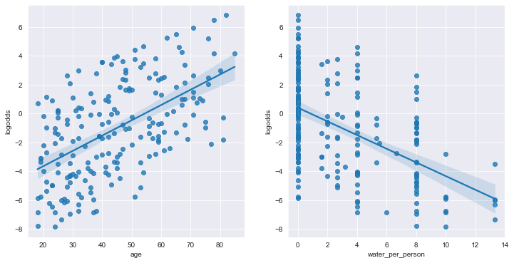
Linearity can be checked by graphing the log-odds of the outcome against each numeric predictor to see if the relationship is linear.

7. Checking model assumptions
The model is statistically significant (c2 = 145.6; p < 0.05), indicating that the variables in the model work together to help explain zombie status. Older age, having no food, living in suburban or urban areas (compared to rural), and having no access to medication increased the odds of being a zombie. Access to sanitation and having enough water decreased the odds of being a zombie. The model correctly predicted the zombie status of 63 zombies and 109 humans, or 172 of the 200 participants. Before relying on the model, check model assumptions: no multicollinearity and linearity.
Checking multicollinearity:
We can use the generalized variance inflation factor (GVIF) to check for multicollinearity. The GVIF determines to what extent each independent variable can be explained by the rest of the independent variables. When an independent variable is well-explained by the other independent variables, the GVIF is high, indicating that the variable is redundant and should be dropped from the model. Values greater than two are often used to indicate a failed multicollinearity assumption.
df = degrees of freedom
Checking linearity:
Linearity can be checked by graphing the log-odds of the outcome against each numeric predictor to see if the relationship is linear.
from statsmodels.stats.outliers_influence import variance_inflation_factor
from patsy import dmatrices

#features = model_var.append('zombie')
y, X = dmatrices(formula, zombies, return_type='dataframe')

vif = pd.DataFrame()
vif['VIF'] = [variance_inflation_factor(X.values,i) for i in range(X.shape[1])]
vif['features'] = X.columns
print(vif, '\n')

if(vif.VIF[1:].all() < 2.5): # the Intercept to be ignored
    print('multicollinearity is not a problem in our model as the Variance Inflation Factor is low for all features')
         VIF                        features
0  13.028386                       Intercept
1   1.277556              C(food)[T.No food]
2   1.202480         C(rurality)[T.Suburban]
3   1.322900            C(rurality)[T.Urban]
4   1.268081  C(medication)[T.No medication]
5   1.090838     C(sanitation)[T.Sanitation]
6   1.045321                             age
7   1.145331                water_per_person

multicollinearity is not a problem in our model as the Variance Inflation Factor is low for all features
plt.figure(figsize=(12,6))
plt.subplot(1,2,1)
sns.regplot(y=zombies['logodds'], x="age", data=zombies)
plt.subplot(1,2,2)
sns.regplot(y=zombies['logodds'], x="water_per_person", data=zombies)
plt.show()
8. Interpreting assumptions and making predictions
We find that the GVIF scores are low, indicating the model meets the assumption of no perfect multicollinearity. The plots show relatively minor deviation from the linearity assumption for age and water.person. The assumptions appear to be sufficiently met.
One of your friends on the analysis team hasn't been able to reach her dad or brother for hours, but she knows that they have food, medicine, and sanitation from an earlier phone conversation. Her 71-year-old dad lives alone in a suburban area and is excellent at preparedness; he has about five gallons of water. Her 40-year-old brother lives in an urban area and estimated three gallons of water per person. She decides to use the model to compute the probability they are zombies.
newdata = pd.DataFrame({'age': [71,40],
                        'water_per_person': [5,3],
                        'food': ['Food', 'Food'],
                        'rurality': ['Suburban', 'Urban'],
                        'medication': ['Medication', 'Medication'],
                        'sanitation': ['Sanitation', 'Sanitation']
                       })

predictions_new = model.predict(newdata)
predictions_new
0    0.154577
1    0.097208
dtype: float64
9. What is your zombie probability?
Her dad has about a 15.5 percent chance of being a zombie and her brother has less than a 10 percent chance. It looks like they are probably safe, which is a big relief! She comes back to the team to start working on a plan to distribute food and common types of medication to keep others safe. The team discusses what it would take to start evacuating urban areas to get people to rural parts of the country where there is a lower percent of zombies. While the team is working on these plans, one thought keeps distracting you…your family may be safe, but how safe are you?
Add your own real-life data to the newdata data frame and predict your own probability of becoming a zombie!
newdata = pd.DataFrame({'age': [71,40,34],
                        'water_per_person': [5,3,1],
                        'food': ['Food', 'Food','Food'],
                        'rurality': ['Suburban', 'Urban','Suburban'],
                        'medication': ['Medication', 'Medication', 'Medication'],
                        'sanitation': ['Sanitation', 'Sanitation', 'Sanitation']
                       })


predictions_new = model.predict(newdata)
predictions_new
0    0.154577
1    0.097208
2    0.027275
dtype: float64
10. Are you ready for the zombie apocalypse?
While it is unlikely to be a zombie apocalypse will happen in the near future, the information presented in this notebook draws on emergency preparedness recommendations from the CDC. Although there is no way to make ourselves younger, we can have food, water, medication, and other supplies ready to ensure we are safe in the event of a blizzard, flood, tornado, or another emergency. After computing your zombie probability, think about what you could personally do to increase the likelihood that you will stay safe in the next storm or zombie apocalypse.
# What is your probability of becoming a zombie?
me = 0.027275

# How prepared are you for a real emergency?
preparedness_level  = "I got this!"
Background Information
That was fun, this project is certainly quite refreshing.
I did not want to change anything on the Original Project by Datacamp, so the goal was to implement just the same with Python and waived initially data wrangling.
Indeed this has been actually an Official CDC campaign as still can be seen on the overview page :

</p>
The CDC have apparently switched off the pages of the 2011 Zombie Apocalypse Preparedness campaign in the meanwhile, still being available earlier this year. This campaign was probably phased out after 10 years running. You can check the content out with the Waybackmachine: https://web.archive.org/web/20210303012528/https://www.cdc.gov/cpr/zombie/index.htm