Applied Multi-Criteria Supplier Selection with Data Envelopment Analysis & Game Cross-Efficiency Model
Data envelopment analysis (DEA) was proposed by Charnes (CCR model) and developed by Banker (BCC model). The DEA method based on the marginal benefit and linear programming theory, through analysing if decision making units (DMUs) are located in production frontier to compare the relative efficiencies among DMUs and shows the respective optimum value. DEA is an approach for measuring the relative efficiency of peer DMUs with multiple inputs and multiple outputs simultaneously. It is a powerful technique used in multi-criteria decision-making, and it plays a significant role in supplier selection as part of supply chain management. DEA is particularly useful in this context because it allows organizations to evaluate and compare multiple suppliers based on various criteria simultaneously. [1]
Critical roles of DEA
-
It allows organizations to assess suppliers based on your own multiple criteria, such as cost, quality, and reliability, simultaneously, providing a holistic view of supplier performance.
-
It ensures objective and data-driven decision-making, reducing bias and enhancing transparency in supplier selection. It helps organizations make choices that align with their strategic objectives.
-
It assists in resource allocation by identifying suppliers that offer the best value for resources invested, leading to cost savings and improved performance.
-
DEA supports risk management by identifying consistently efficient suppliers, which is vital in mitigating potential disruptions in the supply chain.
DEA advantages
- Input and output indicators don’t have to be unified dimension.
- The weights of input and output are determined by solving the linear programming that avoid the effect of human’s subjective determining the weight.
- It does not need to consider the relation between the input and output etc.
In summary, DEA is a valuable tool for multi-criteria decision-making in supplier selection within supply chain management. It enhances supplier evaluation, promotes objectivity, aligns with strategic goals, and supports continuous improvement, ultimately contributing to a more robust and competitive supply chain ecosystem.
DEA is also one of the most used techniques for supplier selection [1]. This blog is about the DEA variant of Game Cross-Efficiency and I like to refer to their article “The DEA Game Cross-efficiency Model for Supplier Selection Problem under Competition”.
Analog to their application of DEA on supplier data, I want to apply this analysis method to another dataset for supplier selection and demonstrate the implementation both with R language as well as Excel Solver/DEA Frontier. The latter for cross checking results, as I am going to use a given R implementation [2] that I can cross-check with the excel results for its validity.
Suppliers are treated as DMUs and competition among the vendors is not considered. This is due to the vendor of DEA models used which only assume some basic relations among the inputs and outputs. When DMUs are viewed as players in a game, cross-efficiency scores may be viewed as payoffs, and each DMU may choose to take a non-cooperative game stance to the extent that it will attempt to maximize its (worst possible) payoff. If one adopts this game theoretic approach, it may be argued that the existing approaches to cross evaluation suffer shortcomings in regard to these common situations. Liang et al. “proposed a DEA game Cross-efficiency approach when competition exists between competition exists between DMUs, and proved that the approach leads to a number of unique Nash equilibrium DEA weights.”[3][1]
Liang defined game cross-efficiency as such: “In a game sense, one player $D M U^{d}$ is given an efficiency score $\alpha_{d}$, and that another player $D M U_{j}$ then tries to maximize its own efficiency, subject to the condition that $\alpha_{d}$ cannot be decreased.”
Game cross-efficiency for $D M U_{j}$ relative to $D M U_{d}$:
\[\alpha_{d j}=\frac{\sum_{r=1}^{s} u_{r j}^{d} y_{r j}}{\sum_{i=1}^{m} v_{i j}^{d} x_{i j}}, d=1,2, \cdots, n,\]For each $D M U_{j}$, the game d-cross efficiency can be calculated [15]:
\[\begin{aligned} & \operatorname{Max} \quad \sum_{r=1}^{s} u_{r j}^{d} y_{r j} \\ & \operatorname{s.t}\left\{\begin{array}{l} \sum_{i=1}^{m} v_{i j}^{d} x_{i l}-\sum_{r=1}^{s} u_{r j}^{d} y_{r l} \geq 0, l=1,2, \cdots, n, \\ \sum_{i=1}^{m} v_{i j}^{d} x_{i j}=1, \\ \alpha_{d} \sum_{i=1}^{m} v_{i j}^{d} x_{i d}-\sum_{r=1}^{s} u_{r j}^{d} y_{r d} \leq 0, \\ v_{i j}^{d} \geq 0, i=1,2, \cdots, m, \\ u_{r j}^{d} \geq 0, r=1,2, \cdots, s . \end{array}\right. \end{aligned}\]Assumed the optimal solution of aboves model as $u_{r j}^{d^{*}}\left(\alpha_{d}\right)$, for each $D M U_{j}$, the average game cross-efficiency formulated as:
\[\alpha_{j}=\frac{1}{n} \sum_{d=1}^{n} \sum_{r=1}^{s} u_{r j}^{d^{*}}\left(\alpha_{d}\right) y_{r j}\][1]
DEA game cross-efficiency with R
#install.packages("xlsx")
#install.packages("lpSolve")
#install.packages("Benchmarking")
### libraries

library(xlsx)
library(lpSolve)
library(utils)
library(Benchmarking)


### importing data from excel check value format or class

#data=read.xlsx("supplier-selection-gamecross-matrix-for-R.xlsx",sheet = "Ma", header=TRUE,startRow=1, sheetIndex=1) # read spreadsheet
data=read.xlsx("supplier-selection-gamecross-matrix-for-R.xlsx",sheet = "Vörösmarty", header=TRUE,startRow=1, sheetIndex=1) # read spreadsheet

### Cut the name column to create a data matrix
data
| NA. | Leadtime.days. | Quality... | Price... | Reusability... | CO2 |
|---|---|---|---|---|---|
| <chr> | <dbl> | <dbl> | <dbl> | <dbl> | <dbl> |
| DMU1 | 2.0 | 0.013 | 2.0 | 70 | 0.033 |
| DMU2 | 1.0 | 0.014 | 3.0 | 50 | 0.100 |
| DMU3 | 3.0 | 0.011 | 5.0 | 60 | 0.067 |
| DMU4 | 1.5 | 0.012 | 1.0 | 40 | 0.050 |
| DMU5 | 2.5 | 0.013 | 2.5 | 65 | 0.029 |
| DMU6 | 2.0 | 0.011 | 4.0 | 90 | 0.040 |
| DMU7 | 3.0 | 0.013 | 1.5 | 75 | 0.067 |
| DMU8 | 1.5 | 0.012 | 3.5 | 85 | 0.050 |
| DMU9 | 1.0 | 0.014 | 3.5 | 55 | 0.100 |
| DMU10 | 2.5 | 0.013 | 4.0 | 45 | 0.100 |
| DMU11 | 3.5 | 0.011 | 2.5 | 80 | 0.040 |
| DMU12 | 2.0 | 0.015 | 1.5 | 50 | 0.050 |
| DMU13 | 3.0 | 0.012 | 3.0 | 75 | 0.067 |
| DMU14 | 1.5 | 0.014 | 4.5 | 85 | 0.050 |
| DMU15 | 1.0 | 0.015 | 2.0 | 75 | 0.067 |
utility=strsplit(as.character(data[,1]),"_m") # utilityâ???Ts names
utility

data[1] <- NULL
- 'DMU1'
- 'DMU2'
- 'DMU3'
- 'DMU4'
- 'DMU5'
- 'DMU6'
- 'DMU7'
- 'DMU8'
- 'DMU9'
- 'DMU10'
- 'DMU11'
- 'DMU12'
- 'DMU13'
- 'DMU14'
- 'DMU15'
data
| Leadtime.days. | Quality... | Price... | Reusability... | CO2 |
|---|---|---|---|---|
| <dbl> | <dbl> | <dbl> | <dbl> | <dbl> |
| 2.0 | 0.013 | 2.0 | 70 | 0.033 |
| 1.0 | 0.014 | 3.0 | 50 | 0.100 |
| 3.0 | 0.011 | 5.0 | 60 | 0.067 |
| 1.5 | 0.012 | 1.0 | 40 | 0.050 |
| 2.5 | 0.013 | 2.5 | 65 | 0.029 |
| 2.0 | 0.011 | 4.0 | 90 | 0.040 |
| 3.0 | 0.013 | 1.5 | 75 | 0.067 |
| 1.5 | 0.012 | 3.5 | 85 | 0.050 |
| 1.0 | 0.014 | 3.5 | 55 | 0.100 |
| 2.5 | 0.013 | 4.0 | 45 | 0.100 |
| 3.5 | 0.011 | 2.5 | 80 | 0.040 |
| 2.0 | 0.015 | 1.5 | 50 | 0.050 |
| 3.0 | 0.012 | 3.0 | 75 | 0.067 |
| 1.5 | 0.014 | 4.5 | 85 | 0.050 |
| 1.0 | 0.015 | 2.0 | 75 | 0.067 |
#### identify each column by its name to bind them into a datamatrix

#meanmax.=data[,2]
#variancemin.=data[,3]
#skewmax.=data[,4]
#kurtmin.=data[,5]


##### bend all column into data matrix with input first sceeded by the output

#datamatrix=cbind(variancemin.,kurtmin.,meanmax.,skewmax.) # data matrix
#datamatrix
##### add row names companies or DMUs number

#rownames(datamatrix)=utility

#### check the data into a new value

data_dea = as.matrix(data)
rownames(data_dea)=utility
data_dea
| Leadtime.days. | Quality... | Price... | Reusability... | CO2 | |
|---|---|---|---|---|---|
| DMU1 | 2.0 | 0.013 | 2.0 | 70 | 0.033 |
| DMU2 | 1.0 | 0.014 | 3.0 | 50 | 0.100 |
| DMU3 | 3.0 | 0.011 | 5.0 | 60 | 0.067 |
| DMU4 | 1.5 | 0.012 | 1.0 | 40 | 0.050 |
| DMU5 | 2.5 | 0.013 | 2.5 | 65 | 0.029 |
| DMU6 | 2.0 | 0.011 | 4.0 | 90 | 0.040 |
| DMU7 | 3.0 | 0.013 | 1.5 | 75 | 0.067 |
| DMU8 | 1.5 | 0.012 | 3.5 | 85 | 0.050 |
| DMU9 | 1.0 | 0.014 | 3.5 | 55 | 0.100 |
| DMU10 | 2.5 | 0.013 | 4.0 | 45 | 0.100 |
| DMU11 | 3.5 | 0.011 | 2.5 | 80 | 0.040 |
| DMU12 | 2.0 | 0.015 | 1.5 | 50 | 0.050 |
| DMU13 | 3.0 | 0.012 | 3.0 | 75 | 0.067 |
| DMU14 | 1.5 | 0.014 | 4.5 | 85 | 0.050 |
| DMU15 | 1.0 | 0.015 | 2.0 | 75 | 0.067 |
N = dim(data)[1]  # number of DMU

s = 3 # number of inputs

m = 2 # number of outputs

#inputs = as.matrix(data[,c(1:s)])
inputs <- as.matrix(data[,c(1:s)])
rownames(inputs)=utility
inputs
| Leadtime.days. | Quality... | Price... | |
|---|---|---|---|
| DMU1 | 2.0 | 0.013 | 2.0 |
| DMU2 | 1.0 | 0.014 | 3.0 |
| DMU3 | 3.0 | 0.011 | 5.0 |
| DMU4 | 1.5 | 0.012 | 1.0 |
| DMU5 | 2.5 | 0.013 | 2.5 |
| DMU6 | 2.0 | 0.011 | 4.0 |
| DMU7 | 3.0 | 0.013 | 1.5 |
| DMU8 | 1.5 | 0.012 | 3.5 |
| DMU9 | 1.0 | 0.014 | 3.5 |
| DMU10 | 2.5 | 0.013 | 4.0 |
| DMU11 | 3.5 | 0.011 | 2.5 |
| DMU12 | 2.0 | 0.015 | 1.5 |
| DMU13 | 3.0 | 0.012 | 3.0 |
| DMU14 | 1.5 | 0.014 | 4.5 |
| DMU15 | 1.0 | 0.015 | 2.0 |
outputs = as.matrix(data[,c((s+1):(s+m))])
rownames(outputs)=utility
outputs
| Reusability... | CO2 | |
|---|---|---|
| DMU1 | 70 | 0.033 |
| DMU2 | 50 | 0.100 |
| DMU3 | 60 | 0.067 |
| DMU4 | 40 | 0.050 |
| DMU5 | 65 | 0.029 |
| DMU6 | 90 | 0.040 |
| DMU7 | 75 | 0.067 |
| DMU8 | 85 | 0.050 |
| DMU9 | 55 | 0.100 |
| DMU10 | 45 | 0.100 |
| DMU11 | 80 | 0.040 |
| DMU12 | 50 | 0.050 |
| DMU13 | 75 | 0.067 |
| DMU14 | 85 | 0.050 |
| DMU15 | 75 | 0.067 |
#### start of the algorithm

crosseff = matrix(0,nrow=N,ncol=N) # initialize cross efficiency matrix

f.rhs = c(rep(0,(N+s+m)),1) # RHS constraints

f.dir = c(rep("<=",N),rep(">",(s+m)),"=") # directions of the constraints

aux = cbind(-1*inputs,outputs) # matrix of constraint coefficients in (CCR)
aux11= rbind(aux,diag(s+m))

for (i in 1:N) {

  f.obj = c(rep(0,s),t(outputs[i,])) # objective function coefficients

  f.con = rbind(aux11 ,c(inputs[i,(1:s)], rep(0,m))) # add LHS

  results = lp("max",f.obj,f.con,f.dir,f.rhs,scale=1,compute.sens=TRUE) # solve LPP

  multipliers = results$solution # input and output weights

  efficiency = results$objval # efficiency score

  duals = results$duals # shadow prices

  #### keep weight and final efficiency (CCR) values

  if (i==1) {

    weights = c(multipliers[seq(1,s+m)])

    effcrs = efficiency

    lambdas = duals [seq(1,N)]

  } else {

    weights = rbind(weights,c(multipliers[seq(1,s+m)]))

    effcrs = rbind(effcrs , efficiency)

    lambdas = rbind(lambdas,duals[seq(1,N)])

  }
  ##### fill in the cross efficiency matrix

  for (j in 1:N) {

    crosseff[i,j] = multipliers[(s+1):(m+s)]%*%(outputs[j,])/(multipliers[1:s]%*%(inputs[j,]))

  }

}
set_plot_dimensions <- function(width_choice, height_choice) {
options(repr.plot.width=width_choice, repr.plot.height=height_choice)
}
set_plot_dimensions(10, 10)
# A quick frontier with 1 input and 1 output
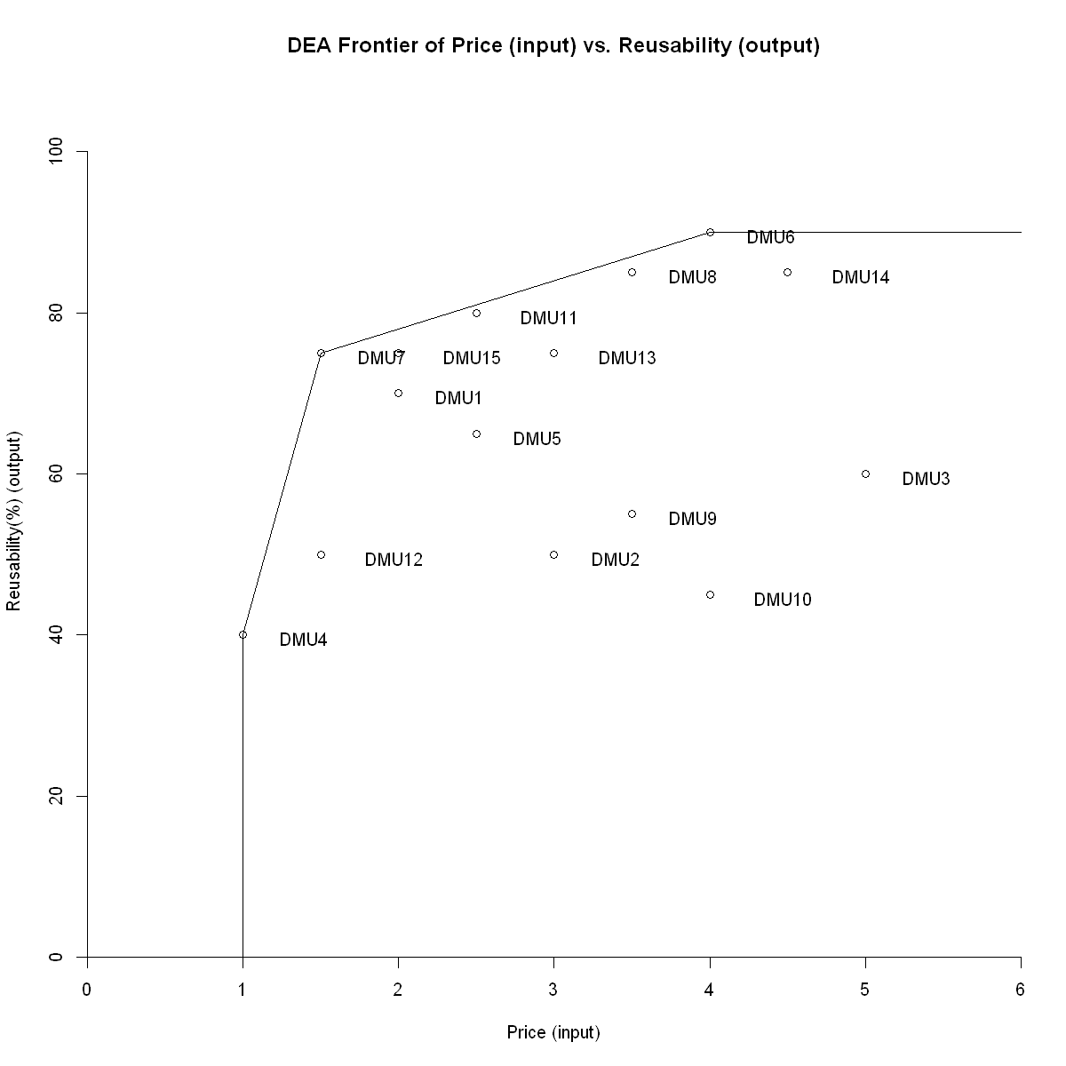
dea.plot(inputs[,3],outputs[,1], main="DEA Frontier of Price (input) vs. Reusability (output)", txt=TRUE, xlab="Price (input)", ylab="Reusability(%) (output)")
#dea.plot.frontier(x,y,txt=TRUE)
#dea.plot.isoquant(inputs[,1], inputs[,2], RTS="crs", txt=TRUE)
#dea.plot.transform(outputs[,1], outputs[,2], RTS="crs", txt=TRUE)
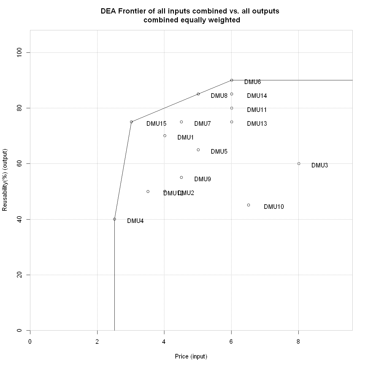
dea.plot(inputs,outputs, GRID=TRUE, main="DEA Frontier of all inputs combined vs. all outputs \n combined equally weighted", txt=TRUE, xlab="Price (input)", ylab="Reusability(%) (output)")
#### create a matrix with CCR Efficiencies and relevant weights, we can add the lamdas (shadow prices)

matrix_results = cbind(effcrs,weights)

rownames(matrix_results) = rownames(data_dea)

colnames(matrix_results) = c("efficiency",colnames(data_dea)[1:(s+m)])

#### Compute the mean Cross Efficiences

rankingb = (N*apply(crosseff,2,mean))/(N) #mean CrossEff including self apparaisal

rankinga = (N*apply(crosseff,2,mean)-diag(crosseff))/(N-1)  #mean CrossEff without self apparaisal

maverick = (effcrs-rankingb)/rankingb # index developed by Green et al with self apparaisal


mavericka = (effcrs-rankinga)/rankinga # index developed by Green et al without self apparaisal

Table = t(rbind(as.numeric(effcrs),round(rankingb,4),t(maverick))) # Table with CCR, meanCrosseff and the maverick index with self apparaisal this will later be used for the game cross effeciency

colnames(Table) = c('CCR','cross_eff','Maverick')

rownames(Table) = rownames(data_dea)

Tablef = t(rbind(as.numeric(effcrs),round(rankingb,4),t(maverick))) # Table with CCR, meanCrosseff and the maverick index with self apparaisal this will later be used for final comparaison

colnames(Tablef) = c('CCR','cross_eff','Maverick')

rownames(Tablef) = rownames(data_dea)

Tabl = t(rbind(as.numeric(effcrs),rankinga,t(mavericka)))# Table with CCR, meanCrosseff and the maverick index without self apparaisal

colnames(Tabl) = c('CCR','cross_eff','Maverick')

rownames(Tabl) = rownames(data_dea)

Table

Arbitrary=Table[,2]
| CCR | cross_eff | Maverick | |
|---|---|---|---|
| DMU1 | 0.9382781 | 0.7273 | 0.29012551 |
| DMU2 | 1.0000000 | 0.7282 | 0.37328098 |
| DMU3 | 0.9908787 | 0.5189 | 0.90971973 |
| DMU4 | 1.0000000 | 0.6926 | 0.44382622 |
| DMU5 | 0.7829766 | 0.5870 | 0.33389454 |
| DMU6 | 1.0000000 | 0.7784 | 0.28473576 |
| DMU7 | 1.0000000 | 0.8436 | 0.18543135 |
| DMU8 | 1.0000000 | 0.8328 | 0.20077036 |
| DMU9 | 1.0000000 | 0.7370 | 0.35687535 |
| DMU10 | 1.0000000 | 0.5156 | 0.93961001 |
| DMU11 | 1.0000000 | 0.7144 | 0.39971783 |
| DMU12 | 0.7827103 | 0.6092 | 0.28485513 |
| DMU13 | 1.0000000 | 0.7035 | 0.42151975 |
| DMU14 | 0.9419525 | 0.7171 | 0.31351867 |
| DMU15 | 1.0000000 | 0.9655 | 0.03573689 |
#########agressive cross efficiency######################

eff = matrix(0,nrow=N,ncol=N) # initialize cross efficiency matrix


for (i in 1:N) {

  f.rhs = c(rep(0,(N+1)),rep(0,(s+m)),1) # RHS constraints

  f.dir = c(rep("<=",N),"=",rep(">",(s+m)),"=") # directions of the constraints

  aux = cbind(-1*inputs,outputs) # matrix of constraint coefficients in (6)

  f.obj = c(rep(0,s),t(outputs[i,])) # objective function coefficients

  for (u in 1:N) {

    alpha=Table[u,1]

    aux1 = rbind(aux ,c(alpha*inputs[u,],-1*outputs[u,])) # add LHS

    aux11=rbind(aux1,diag(s+m))

    f.con = rbind(aux11 ,c(inputs[i,], rep(0,m))) # add LHS

    results = lp("min",f.obj,f.con,f.dir,f.rhs,scale=1,compute.sens=TRUE) # solve LPP

    Gmultipliers = results$solution # input and output weights

    eff[u,i]=results$objval

  }

}


agressive = (N*apply(eff,2,mean))/(N)

agCross=eff
#########benevolant cross efficiency######################

eff = matrix(0,nrow=N,ncol=N) # initialize cross efficiency matrix


for (i in 1:N) {

  f.rhs = c(rep(0,(N+1)),rep(0,(s+m)),1) # RHS constraints

  f.dir = c(rep("<=",N),"=",rep(">",(s+m)),"=") # directions of the constraints

  aux = cbind(-1*inputs,outputs) # matrix of constraint coefficients in (6)

  f.obj = c(rep(0,s),t(outputs[i,])) # objective function coefficients

  for (u in 1:N) {

    alpha=Table[u,1]

    aux1 = rbind(aux ,c(alpha*inputs[u,],-1*outputs[u,])) # add LHS

    aux11=rbind(aux1,diag(s+m))

    f.con = rbind(aux11 ,c(inputs[i,], rep(0,m))) # add LHS

    results = lp("max",f.obj,f.con,f.dir,f.rhs,scale=1,compute.sens=TRUE) # solve LPP

    Gmultipliers = results$solution # input and output weights

    eff[u,i]=results$objval

  }

}


benevolant = (N*apply(eff,2,mean))/(N)

benCross=eff
#########Game cross efficiency######################

eps=0.0001 ## small value to be chosen by the author
z = 0 # counter
#iteration_list <- vector(mode='list', length=2)
iter_df <- data.frame(x=integer(),
                      i=integer(),
                      u=integer(),
                      gameff=double()
                     )

Table = t(rbind(as.numeric(effcrs),rankingb,t(maverick)))
eff = matrix(0,nrow=N,ncol=N) # initialize cross efficiency matrix

Table_2 = matrix(0,nrow=N,ncol=3) # initialize cross efficiency matrix


for (x in 1:N) {

  while  (abs(Table[x,2]-Table_2[x,2])>=eps) {

    for (i in 1:N) {

      f.rhs = c(rep(0,(N+1)),rep(0,(s+m)),1) # RHS constraints

      f.dir = c(rep("<=",(N+1)),rep(">",(s+m)),"=") # directions of the constraints

      aux = cbind(-1*inputs,outputs) # matrix of constraint coefficients in (6)

      f.obj = c(rep(0,s),t(outputs[i,])) # objective function coefficients

      for (u in 1:N) {

        alpha=Table[u,2]

        aux1 = rbind(aux ,c(alpha*inputs[u,],-1*outputs[u,])) # add LHS

        aux11=rbind(aux1,diag(s+m))

        f.con = rbind(aux11 ,c(inputs[i,], rep(0,m))) # add LHS

        results = lp("max",f.obj,f.con,f.dir,f.rhs,scale=1,compute.sens=TRUE) # solve LPP

        Gmultipliers = results$solution # input and output weights

        gameff = results$objval # game efficiency score

        eff[u,i]=results$objval

      }

    }

    Table_2=Table

    rankingg = (N*apply(eff,2,mean))/(N)

    Table[,2]=t(round(rankingg,4))

    colnames(Table) = c('CCR','cross_eff','Maverick')

    rownames(Table) = rownames(data_dea)

    colnames(Table_2) = c('CCR','game_cross_eff','Maverick')

    rownames(Table_2) = rownames(data_dea)


  }
}
CCR=Table[,1]

Game_cross_eff=Table[,2]

Cross_eff=Tablef[,2]

Final_Table=cbind(CCR, Cross_eff, Game_cross_eff ) # final results

rownames(Final_Table) = rownames(data_dea)

colnames(crosseff)=utility

colnames(eff)=utility

rownames(crosseff)=utility

rownames(eff)=utility

Cross_efficiency_matrix=crosseff

Game_Cross_efficiency_matrix=eff

CCR=Table[,1]

Game_cross=Final_Table[,3]


Table_resume=cbind(CCR,Arbitrary,agressive,benevolant,Game_cross)

Table_resume
| CCR | Arbitrary | agressive | benevolant | Game_cross | |
|---|---|---|---|---|---|
| DMU1 | 0.9382781 | 0.7273 | 0.5587422 | 0.8130956 | 0.8689 |
| DMU2 | 1.0000000 | 0.7282 | 0.6774460 | 0.8855876 | 0.9652 |
| DMU3 | 0.9908787 | 0.5189 | 0.4801841 | 0.7704103 | 0.8694 |
| DMU4 | 1.0000000 | 0.6926 | 0.5821754 | 0.7921313 | 0.8468 |
| DMU5 | 0.7829766 | 0.5870 | 0.4609819 | 0.6793966 | 0.7253 |
| DMU6 | 1.0000000 | 0.7784 | 0.6455886 | 0.9145653 | 0.9630 |
| DMU7 | 1.0000000 | 0.8436 | 0.7094185 | 0.9621560 | 0.9967 |
| DMU8 | 1.0000000 | 0.8328 | 0.6981011 | 0.9329601 | 0.9737 |
| DMU9 | 1.0000000 | 0.7370 | 0.6770268 | 0.8873551 | 0.9637 |
| DMU10 | 1.0000000 | 0.5156 | 0.4940107 | 0.8020333 | 0.9097 |
| DMU11 | 1.0000000 | 0.7144 | 0.5790230 | 0.8758740 | 0.9454 |
| DMU12 | 0.7827103 | 0.6092 | 0.5065629 | 0.6760489 | 0.7103 |
| DMU13 | 1.0000000 | 0.7035 | 0.6196526 | 0.8979536 | 0.9632 |
| DMU14 | 0.9419525 | 0.7171 | 0.5943811 | 0.8128711 | 0.8586 |
| DMU15 | 1.0000000 | 0.9655 | 0.8033254 | 0.9665137 | 0.9911 |
Table_resume = round(Table_resume, digits = 6)
Table_ranking = cbind(rank(-round(CCR, digits = 6), ties.method = "min"),
                      rank(-Arbitrary, ties.method = "min"),
                      rank(-agressive, ties.method = "min"),
                      rank(-benevolant, ties.method = "min"),
                      rank(-Game_cross, ties.method = "min"))
colnames(Table_ranking) = colnames(Table_resume)
Table_ranking
| CCR | Arbitrary | agressive | benevolant | Game_cross | |
|---|---|---|---|---|---|
| DMU1 | 13 | 7 | 11 | 9 | 11 |
| DMU2 | 1 | 6 | 4 | 7 | 4 |
| DMU3 | 11 | 14 | 14 | 13 | 10 |
| DMU4 | 1 | 11 | 9 | 12 | 13 |
| DMU5 | 14 | 13 | 15 | 14 | 14 |
| DMU6 | 1 | 4 | 6 | 4 | 7 |
| DMU7 | 1 | 2 | 2 | 2 | 1 |
| DMU8 | 1 | 3 | 3 | 3 | 3 |
| DMU9 | 1 | 5 | 5 | 6 | 5 |
| DMU10 | 1 | 15 | 13 | 11 | 9 |
| DMU11 | 1 | 9 | 10 | 8 | 8 |
| DMU12 | 15 | 12 | 12 | 15 | 15 |
| DMU13 | 1 | 10 | 7 | 5 | 6 |
| DMU14 | 12 | 8 | 8 | 10 | 12 |
| DMU15 | 1 | 1 | 1 | 1 | 2 |
# rounding errors produced CCR values beyond value 1
Table_resume["DMU11",1] > Table_resume["DMU10",1]
FALSE
Table_resume["DMU11",1] - Table_resume["DMU10",1]
0
# https://stackoverflow.com/questions/14290364/create-heatmap-with-values-from-matrix-in-ggplot2

#install.packages('pheatmap') # if not installed already
library(pheatmap)
set_plot_dimensions(15, 15)
pheatmap(Table_ranking,
         display_numbers = T,
         color = colorRampPalette(c('green','white'))(100),
         cluster_rows = F,
         cluster_cols = F,
         fontsize =20,
         fontsize_number = 20,
         angle_col = 45,
         main="Comparison of DMU game efficiency rankings \n by applied model (lower is better)"
        )
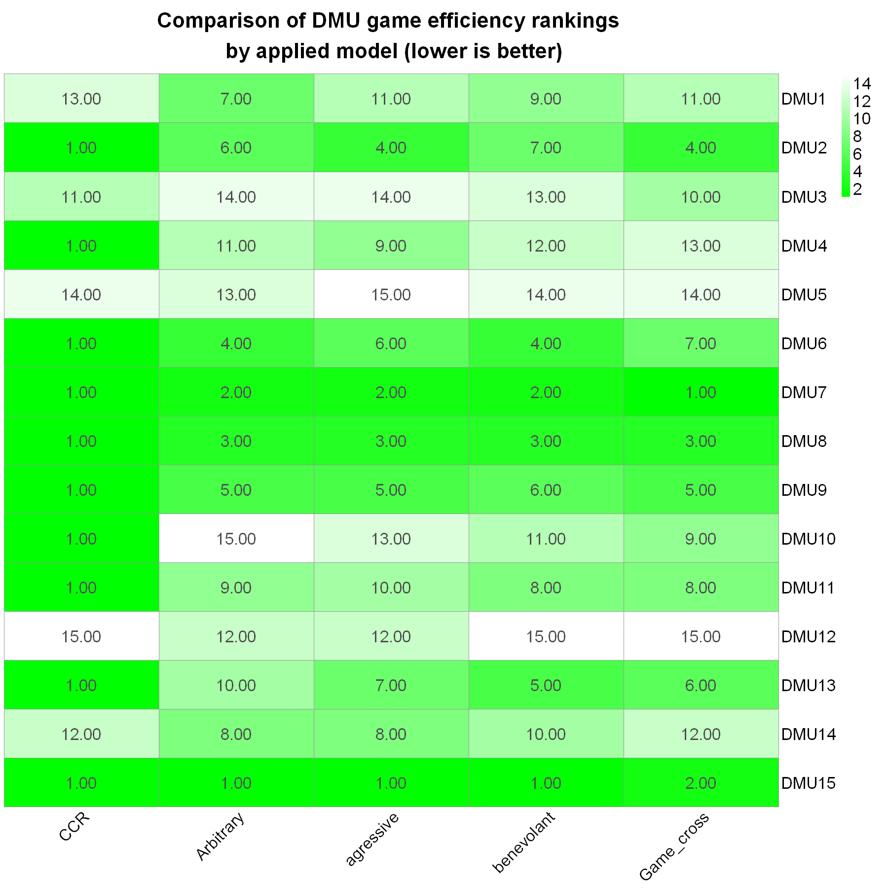
While DMU15 may have been identified as the winner in CCR (with admittedly low discriminatory power), Arbitrary, Agressive & benevolant strategies, it is actually DMU7/Supplier 7 that prevails with the highest game efficiency and rank number #1. Our pick from this analysis.
DEA game cross-efficiency with Excel Solver/DEAFrontier as Cross Check
Running the same data with a Excel solver implementation used in [4], namely the DEAFrontier macro addin yields the exact same results yet with much longer runtime. So this R code is much preffered in running this and more complex problems with higher DMU and variable counts, while DEAFrontier DEA Add-In for Microsoft Excel in its version for Academic Use seems to be limited to 50 DMUs. This limitation by licence is obsolete nowadays, as anybody wanted to opt for efficient software running larger problems.
Bottom line: Identical results.


Conclusion
I used Game DEA to rank the suppliers for their game cross-efficiency, which is a method is particularly well suited to be applied in a competitive environment. Unlike traditional DEA methods for self-assessment and also cross efficiency evaluation methods for peer evaluation, the DEA game cross-efficiency does not produce multiple optimal solutions (see ranking table for no shared ranks in column Game_cross) and is less random and unstable [1].
There are newer DEA models that look at interesting aspects of such a multi criteria decision problem that I may want to apply soon as well:
For instance Imprecise Data Envelopment Analysis (IDEA), which allows cardinal, ordinal or even fuzzy data to be incorporated. In supplier selection this is often the case that no hard data may be available, but e.g. expert rankings of supplier capabilities could be made manually with e.g. a LIKERT scale in place of unavailable data and still could be an essential part of DEA. [5][6]
Or the DEA model with Economic Order Quantity (EOQ)-type inventory costs extending common TCO concepts and also looking at the functional relationship between the input and output criterion values and their efficiency by Dobos and Vörösmarty [7] [8].
References
[3] L. Liang, J. Wu, W. D. Cook and J. Zhu, Operations Research, 56, (2008)
[4] [Zhu, Joe. (2009). Quantitative models for performance evaluation and benchmarking. Data envelopment analysis with spreadsheets. 3rd ed. 10.1007/978-0-387-85982-8. ]
[5] [Zhu, J. (2003). Imprecise data envelopment analysis (IDEA): A review and improvement with an application. Eur. J. Oper. Res., 144, 513-529.